Observation Weights for Differential Abundance of Zero-Inflated Microbiome Data with DESeq2
I recently read through Calgaro et. al. “Assessment of statistical methods from single cell, bulk RNA-seq, and metagenomics applied to microbiome data” where they examined the performance of statistical models developed for bulk RNA (RNA-seq), single-cell RNA-seq (scRNA-seq), and microbial metagenomics to:
- detect differently abundant features (i.e., species or OTUs)
- control false discovery rates
- enhance statistical power
- demonstrate concordance/reproducibility of results.
The analysis was quite impressive (and extensive) with the authors examining 18 different models and 100 whole genome shotgun metagenomic (WMS) or 16S datasets, as well as conducting numerous simulations etc. Given tools developed for RNA-seq data have performed reasonably well on microbiome data, and that both WMS and 16S data is expected to be more sparse (i.e., greater fraction of zero counts) than scRNA-seq data, one might expect approaches for scRNA-seq to outperform methods for bulk RNA and to perhaps do as well those specifically developed for microbiome studies.
Overall, the results of this work suggested that no method outperformed all others under the conditions tested (as we might have come to expect), that compositional data analysis (CODA) methods did not outperform count-based models, and that single-cell approaches did not universally outperform methods for bulk RNA (as has been reported for RNA-seq data here and here). However, zero-inflated count models did appear to provide a better fit for WSM datasets displaying a bimodal distribution (i.e., point mass at zero and second mass separate from zero). Thus, there may be some instances where we might prefer to use count models to analyze microbiome data and to account for the zero-inflation.
So what is zero-inflation when modeling count data and why to do I care? Zero-inflation is the presence of zeros in excess of that expected under a given count distribution (i.e., Poisson or negative binomial). Van den Berge et.al. provide a nice discussion of how zero-inflation leads to increased estimates of variance and how ignoring excess zeros can lead to overestimation of dispersion and subsequent reduction in statistical power to detect differentially abundant features. I highly recommend giving this paper and the original ZINB-Wave paper by Risso et. al. a read for some background. By using observation weights, one can downweight the excess zeros, correct mean-variance estimates, and recover statistical power.
There are several great resources and tutorials describing how to implement these models in R. I have provided some links below. The example I provide uses observation weights with DESeq2, although other approaches can be used. I do not go into much detail here since all of this is well-covered in the linked tutorials (I am basically just applying the workflow to a WMS example):
- Mike Love’s zinbwave-deseq2 tutorial
- Davide Risso’s: An introduction to ZINB-WaVE
- DESeq2 vignette recommendations for single-cell analysis
- Aaron Lun’s: Using scran to analyze single-cell RNA-seq data
One could also model the data using zero-inflated count models such as the zero-inflated negative binomial (ZINB) model or hurdle models directly. An excellent discussion and code to apply this approach is provided in Chapter 12 of the Statistical Analysis of Microbiome Data in R textbook by Xia, Sun, and Chen (2018). One can also fit these types models using MaAsLin2 for example.
Below we will calculate zero inflation weights using the r packages zinbwave and scran and then perform DA testing using DESeq2. The data used here are described in Dhakhan et. al. and are available as part of the curatedMetagenomicData package. We will look to see if we can detect species differing between samples collected from participants in Southern India (Kerala) compared to North-Central India (Bhopal). We first fit the moderated negative binomial model without accounting for the excess zeros and then apply the zero-inflation weights. Filtering of rare taxa is applied before fitting the models.
Loading required libraries
library(tidyverse); packageVersion("tidyverse") ## [1] '1.3.0'library(curatedMetagenomicData); packageVersion("curatedMetagenomicData") ## [1] '1.18.2'library(phyloseq); packageVersion("phyloseq") ## [1] '1.32.0'library(DESeq2); packageVersion("DESeq2") ## [1] '1.28.1'library(apeglm); packageVersion("apeglm") ## [1] '1.10.0'library(zinbwave); packageVersion("zinbwave") ## [1] '1.10.1'library(scran); packageVersion("scran") ## [1] '1.16.0'library(cowplot); packageVersion("cowplot") ## [1] '1.1.0'library(VennDiagram); packageVersion("VennDiagram") ## [1] '1.6.20'library(pscl); packageVersion("pscl") ## [1] '1.5.5'library(MASS); packageVersion("MASS") ## [1] '7.3.51.6'Reading in Dhakan data and converting to phyloseq object
dhakan_eset <- DhakanDB_2019.metaphlan_bugs_list.stool()## snapshotDate(): 2020-04-27## see ?curatedMetagenomicData and browseVignettes('curatedMetagenomicData') for documentation## loading from cache(ps <- ExpressionSet2phyloseq(dhakan_eset,
simplify = TRUE,
relab = FALSE,
phylogenetictree = TRUE))## phyloseq-class experiment-level object
## otu_table() OTU Table: [ 233 taxa and 110 samples ]
## sample_data() Sample Data: [ 110 samples by 20 sample variables ]
## tax_table() Taxonomy Table: [ 233 taxa by 8 taxonomic ranks ]
## phy_tree() Phylogenetic Tree: [ 233 tips and 232 internal nodes ]tax_table(ps) %>%
data.frame() %>%
dplyr::slice(1:5) ## Kingdom Phylum Class
## s__Methanobrevibacter_smithii Archaea Euryarchaeota Methanobacteria
## s__Megamonas_hypermegale Bacteria Firmicutes Negativicutes
## s__Megamonas_funiformis Bacteria Firmicutes Negativicutes
## s__Megamonas_rupellensis Bacteria Firmicutes Negativicutes
## s__Selenomonas_bovis Bacteria Firmicutes Negativicutes
## Order Family
## s__Methanobrevibacter_smithii Methanobacteriales Methanobacteriaceae
## s__Megamonas_hypermegale Selenomonadales Veillonellaceae
## s__Megamonas_funiformis Selenomonadales Veillonellaceae
## s__Megamonas_rupellensis Selenomonadales Veillonellaceae
## s__Selenomonas_bovis Selenomonadales Veillonellaceae
## Genus Species
## s__Methanobrevibacter_smithii Methanobrevibacter Methanobrevibacter_smithii
## s__Megamonas_hypermegale Megamonas Megamonas_hypermegale
## s__Megamonas_funiformis Megamonas Megamonas_funiformis
## s__Megamonas_rupellensis Megamonas Megamonas_rupellensis
## s__Selenomonas_bovis Selenomonas Selenomonas_bovis
## Strain
## s__Methanobrevibacter_smithii <NA>
## s__Megamonas_hypermegale <NA>
## s__Megamonas_funiformis <NA>
## s__Megamonas_rupellensis <NA>
## s__Selenomonas_bovis <NA>tax_table(ps) %>%
data.frame() %>%
dplyr::count(Strain) ## Strain n
## 1 <NA> 233head(taxa_names(ps)) ## [1] "s__Methanobrevibacter_smithii" "s__Megamonas_hypermegale"
## [3] "s__Megamonas_funiformis" "s__Megamonas_rupellensis"
## [5] "s__Selenomonas_bovis" "s__Mitsuokella_multacida"taxa_names(ps) <- gsub("s__", "", taxa_names(ps)) #removing s__ in OTU names)
head(taxa_names(ps))## [1] "Methanobrevibacter_smithii" "Megamonas_hypermegale"
## [3] "Megamonas_funiformis" "Megamonas_rupellensis"
## [5] "Selenomonas_bovis" "Mitsuokella_multacida"otu_table(ps)[1:10, 1:5] ## OTU Table: [10 taxa and 5 samples]
## taxa are rows
## DHAK_HAK DHAK_HAJ DHAK_HAI DHAK_HAH
## Methanobrevibacter_smithii 76500 0 0 0
## Megamonas_hypermegale 0 0 129501 15951
## Megamonas_funiformis 0 0 5009 0
## Megamonas_rupellensis 0 0 2976 609
## Selenomonas_bovis 0 0 0 0
## Mitsuokella_multacida 17171 27663 0 0
## Phascolarctobacterium_succinatutens 22468 0 0 0
## Acidaminococcus_fermentans 0 0 6864 0
## Acidaminococcus_intestini 0 0 929 0
## Megasphaera_elsdenii 0 0 0 0
## DHAK_HAG
## Methanobrevibacter_smithii 37331
## Megamonas_hypermegale 0
## Megamonas_funiformis 0
## Megamonas_rupellensis 0
## Selenomonas_bovis 0
## Mitsuokella_multacida 0
## Phascolarctobacterium_succinatutens 417095
## Acidaminococcus_fermentans 0
## Acidaminococcus_intestini 0
## Megasphaera_elsdenii 0sample_variables(ps) ## [1] "subjectID" "body_site"
## [3] "antibiotics_current_use" "study_condition"
## [5] "disease" "age"
## [7] "infant_age" "age_category"
## [9] "gender" "BMI"
## [11] "country" "location"
## [13] "non_westernized" "DNA_extraction_kit"
## [15] "number_reads" "number_bases"
## [17] "minimum_read_length" "median_read_length"
## [19] "curator" "NCBI_accession"table(sample_data(ps)$location) ##
## Bhopal Kerala
## 53 57sample_data(ps)$location <- factor(sample_data(ps)$location, levels = c("Bhopal", "Kerala"))We can see that we have:
- taxa table with 8 ranks
- strain classification is missing so returns species as OTU names
- can see estimated counts are returned
- there are 20 metadata fields available
- there are n=110 participants (Bhopal = 53 and Kerala = 57)
Filtering low prevalence taxa
The species matrix is very sparse (~84% zeros). I am dropping taxa not seen in at least 20% of samples as we are interested in associations for more prevalent taxa. We would expect to have low power to detect associations for rare taxa and this type of independent filtering will reduce the number of “lower power” tests considered when applying the FDR correction.
species_counts_df <- data.frame(otu_table(ps))
(sum(colSums(species_counts_df == 0))) / (nrow(species_counts_df) * ncol(species_counts_df))
## [1] 0.8353102(ps <- filter_taxa(ps, function(x) sum(x > 0) > (0.2*length(x)), TRUE))## phyloseq-class experiment-level object
## otu_table() OTU Table: [ 64 taxa and 110 samples ]
## sample_data() Sample Data: [ 110 samples by 20 sample variables ]
## tax_table() Taxonomy Table: [ 64 taxa by 8 taxonomic ranks ]
## phy_tree() Phylogenetic Tree: [ 64 tips and 63 internal nodes ]rm(species_counts_df)Only 64 species are seen in 20% of samples. This is an unusually small number, and we might want to dig deeper into understanding why (and if this changes our approach), but we will proceed for now and treat this just as an example of how to generate and apply the observation weights.
Assessing zero proportion after filtering
species_counts_df <- data.frame(otu_table(ps))
species_counts_df <- data.frame(t(species_counts_df))

species_counts_df %>%
  mutate_all(function(x) ifelse(x == 0, 1, 0)) %>%
  summarise_all(function(x) mean(x)) %>%
  t(.) %>%
  data.frame(.) %>%
  dplyr::rename("prop_zeros" = ".") %>%
  ggplot(data = ., aes(x = prop_zeros)) + geom_histogram(bins = 50) +
  scale_x_reverse() +
  labs(x = "\nProportion of Zeros for Each Species", y = "Count\n")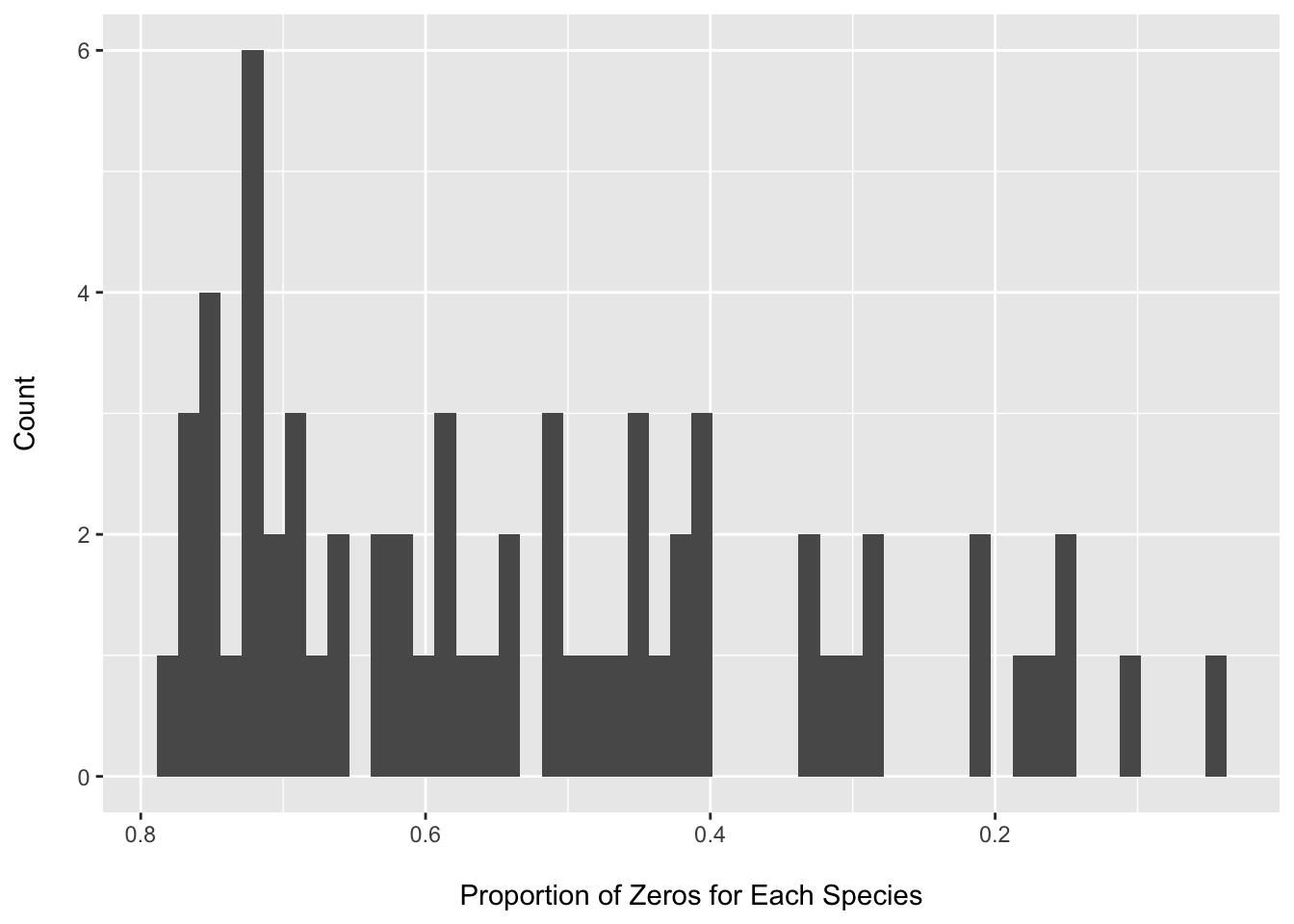
set.seed(123)
species_counts_df %>%
  t(.) %>%
  data.frame(.) %>%
  rownames_to_column(var = "species") %>%
  mutate(rnum = rnorm(n = nrow(.))) %>%
  dplyr::arrange(rnum) %>%
  dplyr::slice(1:12) %>%
  column_to_rownames(var = "species") %>%
  dplyr::select(-rnum) %>%
  t(.) %>%
  data.frame(.) %>%
  pivot_longer(cols = everything(), names_to = "Species", values_to = "Counts") %>%
  dplyr::arrange(Species) %>%
  ggplot(data = ., aes(x = Counts)) + geom_histogram(bins = 100) +
  labs(x = "\nRead Count Distribution", y = "Count\n") +
  facet_wrap(~ Species, scales = "fixed")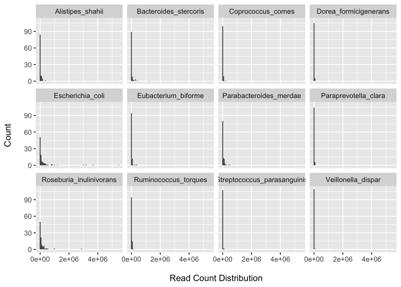
nb1 <- MASS::glm.nb(Escherichia_coli ~ 1, data = species_counts_df)
zinb <- pscl::zeroinfl(Escherichia_coli ~ 1 | 1, data = species_counts_df, dist = "negbin")
BIC(nb1); BIC(zinb)
## [1] 2561.969## [1] 2530.858rm(nb1, zinb, species_counts_df)We can see that there is still a large fraction of zeros after filtering. We can also see that we have large point masses at zero for all the randomly selected species (however we do not see clear bimodal distributions for all).
I provide some code to do a quick comparison of the model fit between the negative binomial and a zero-inflated negative binomial model using the BIC. The zero-inflated model fits the data better for E.coli. More extensive assessment could be done by looking over all taxa and:
- examination of BIC and AIC
- formal testing (i.e., likelihood ratio tests and/or Vuong test
- plotting fitting values from each model and seeing whether they fall along the diagonal (if do not suggest difference between models)
Differential abudnace tetsing via DESeq2 without zero-inflation weights
dds <- phyloseq_to_deseq2(ps, ~ location)## converting counts to integer modedds <- DESeq(dds, test = "Wald", fitType = "local", sfType = "poscounts")## estimating size factors## estimating dispersions## gene-wise dispersion estimates## mean-dispersion relationship## final dispersion estimates## fitting model and testing## -- replacing outliers and refitting for 31 genes
## -- DESeq argument 'minReplicatesForReplace' = 7
## -- original counts are preserved in counts(dds)## estimating dispersions## fitting model and testingplotMA(dds)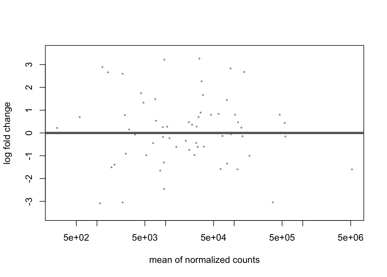
plotDispEsts(dds)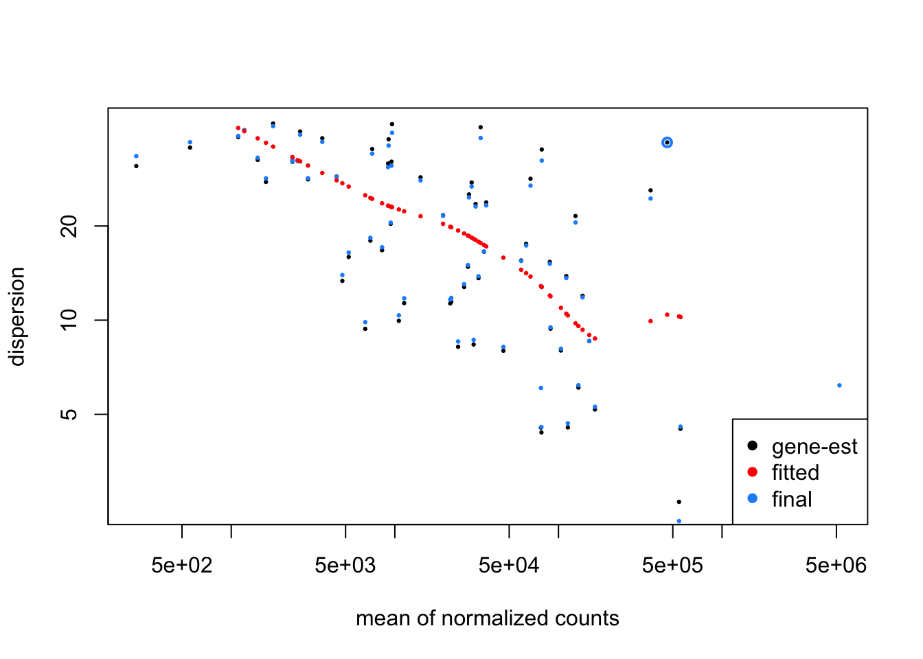
res <- results(dds, cooksCutoff = FALSE)
res
## log2 fold change (MLE): location Kerala vs Bhopal
## Wald test p-value: location Kerala vs Bhopal
## DataFrame with 64 rows and 6 columns
## baseMean log2FoldChange lfcSE stat
## <numeric> <numeric> <numeric> <numeric>
## Megamonas_hypermegale 9535.70 -2.454910 1.53709 -1.5971153
## Megamonas_funiformis 1802.34 -1.389766 1.77764 -0.7818052
## Megamonas_rupellensis 1103.03 -3.086656 1.71482 -1.7999866
## Mitsuokella_multacida 67481.71 -0.132672 1.42818 -0.0928961
## Acidaminococcus_intestini 2638.19 -0.908580 1.72253 -0.5274689
## ... ... ... ... ...
## Sutterella_wadsworthensis 36174.6 -0.599809 1.328139 -0.451617
## Haemophilus_parainfluenzae 21807.9 0.468837 0.939025 0.499280
## Klebsiella_pneumoniae 111591.2 -1.596892 1.016621 -1.570784
## Enterobacter_cloacae 14360.0 -0.611074 1.456008 -0.419692
## Escherichia_coli 167223.9 -1.001510 0.632899 -1.582418
## pvalue padj
## <numeric> <numeric>
## Megamonas_hypermegale 0.1102400 0.495927
## Megamonas_funiformis 0.4343291 0.780820
## Megamonas_rupellensis 0.0718627 0.495927
## Mitsuokella_multacida 0.9259861 0.978360
## Acidaminococcus_intestini 0.5978680 0.927476
## ... ... ...
## Sutterella_wadsworthensis 0.651545 0.927476
## Haemophilus_parainfluenzae 0.617582 0.927476
## Klebsiella_pneumoniae 0.116233 0.495927
## Enterobacter_cloacae 0.674711 0.927476
## Escherichia_coli 0.113554 0.495927df_res <- cbind(as(res, "data.frame"), as(tax_table(ps)[rownames(res), ], "matrix"))
df_res <- df_res %>%
rownames_to_column(var = "OTU") %>%
arrange(padj)
(fdr_otu <- df_res %>%
dplyr::filter(padj < 0.1)) #none with FDR p-val < 0.1## [1] OTU baseMean log2FoldChange lfcSE stat
## [6] pvalue padj Kingdom Phylum Class
## [11] Order Family Genus Species Strain
## <0 rows> (or 0-length row.names)resultsNames(dds)## [1] "Intercept" "location_Kerala_vs_Bhopal"res_LFC <- lfcShrink(dds, coef=2, type="apeglm") #can also consider alternative shrinkage estimator and plot most DE species## using 'apeglm' for LFC shrinkage. If used in published research, please cite:
## Zhu, A., Ibrahim, J.G., Love, M.I. (2018) Heavy-tailed prior distributions for
## sequence count data: removing the noise and preserving large differences.
## Bioinformatics. https://doi.org/10.1093/bioinformatics/bty895plotMA(res_LFC)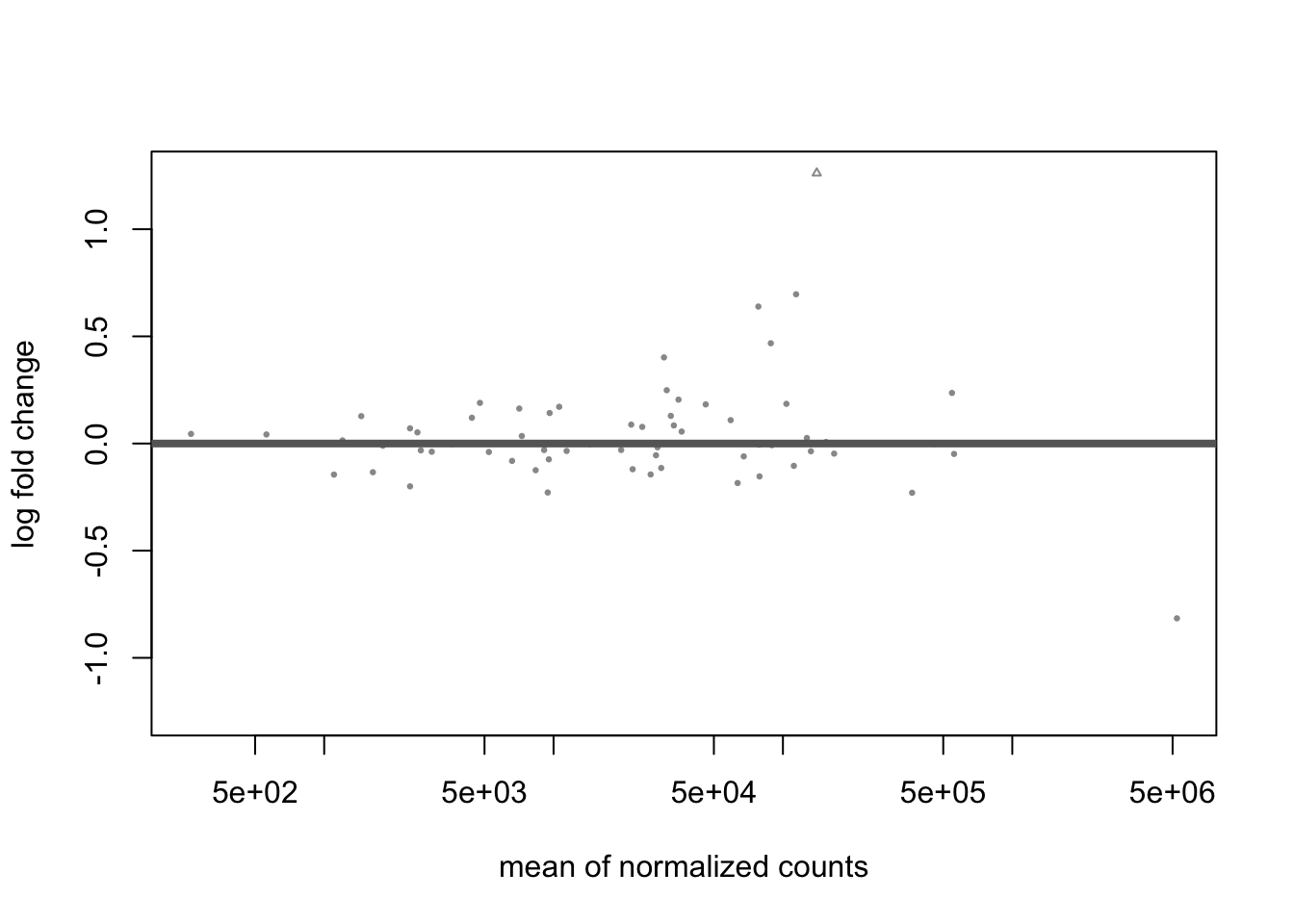
df_res_lfc <- cbind(as(res_LFC, "data.frame"), as(tax_table(ps)[rownames(res_LFC), ], "matrix"))
df_res_lfc <- df_res_lfc %>%
  rownames_to_column(var = "OTU") %>%
  arrange(desc(log2FoldChange))

lfc_otu <- df_res_lfc %>%
  filter(abs(log2FoldChange) > 1) %>%
  droplevels() %>%
  arrange(desc(log2FoldChange))

ggplot(lfc_otu, aes(x = Species, y = log2FoldChange, color = Species)) +
  geom_point(size = 4) +
  labs(y = "\nLog2 Fold-Change for Kerala vs. Bhopal", x = "") +
  theme(axis.text.x = element_text(color = "black", size = 12),
        axis.text.y = element_text(color = "black", size = 12),
        axis.title.y = element_text(size = 14),
        axis.title.x = element_text(size = 14),
        legend.text = element_text(size = 12),
        legend.title = element_text(size = 12),
        legend.position = "none") +
  coord_flip() +
  geom_hline(yintercept = 0, linetype="dotted")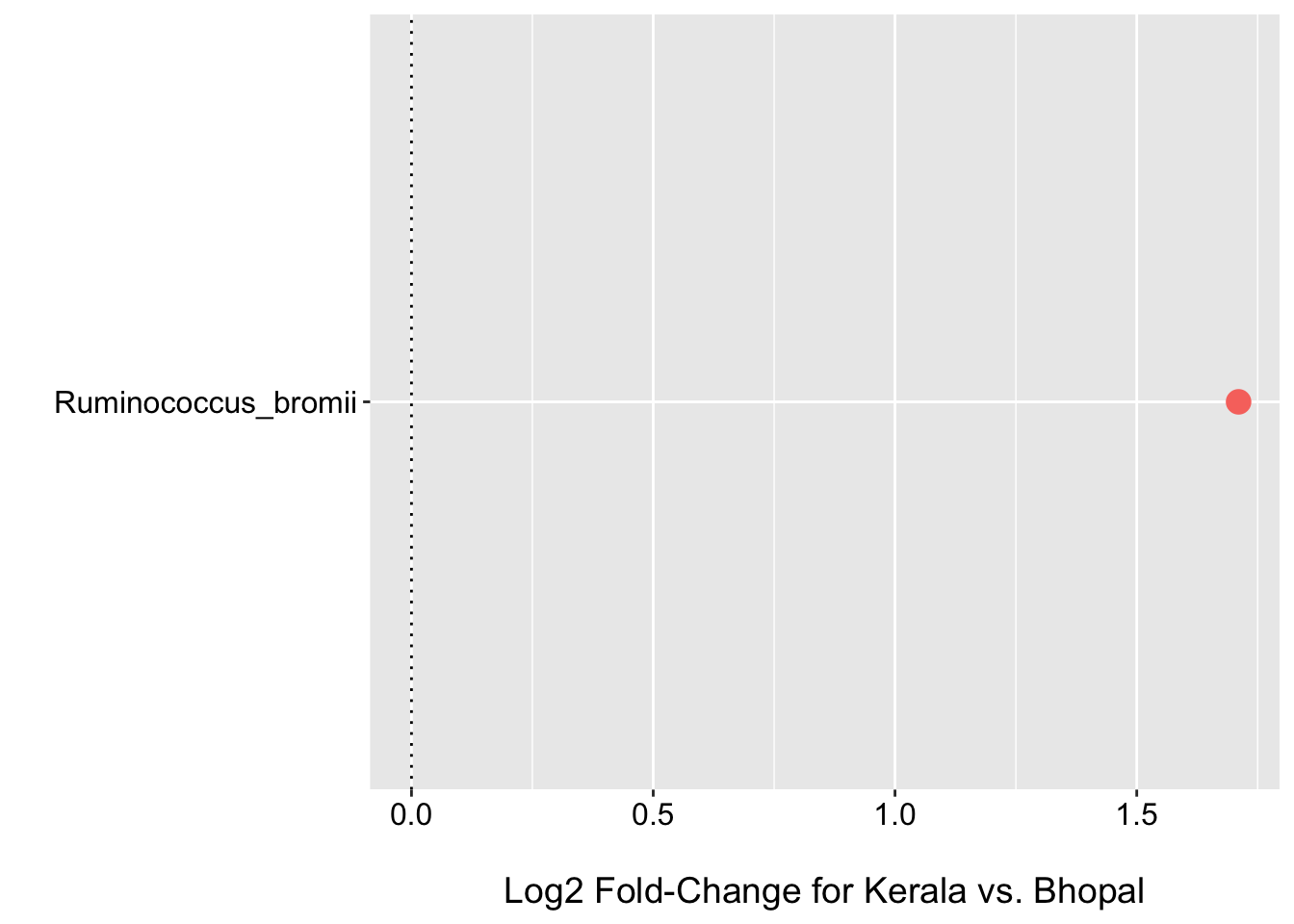
d <- plotCounts(dds, gene = "Ruminococcus_bromii", intgroup = "location", returnData = TRUE)
ggplot(d, aes(x = location, y = count, color = location)) +
  geom_point(position = position_jitter(w = 0.1, h = 0)) +
  labs(x = "", y = "Count\n")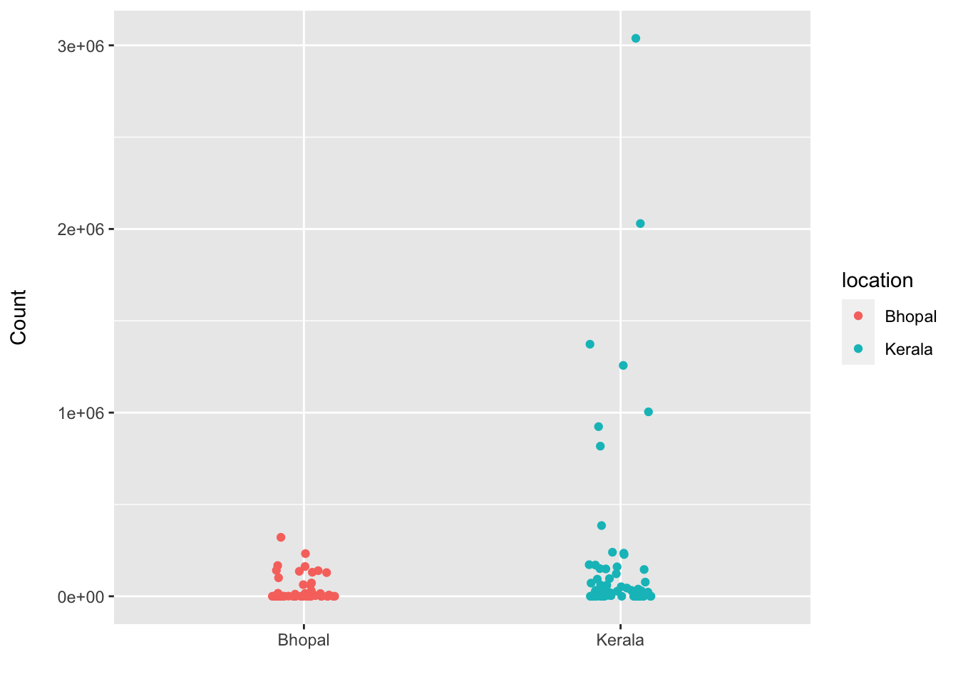
We can see that:
- MA and dispersion trend plots look reasonable
- No species have FDR p-value < 0.1
- Applying shrinkage via the default apeglm approach shrinks most estimates towards zero and only one species R.bromii has a log2 fold-change +/- 1.
- Plot of normalized values also supports higher mean abundance of R.bromii in Kerala
Extending DESeq2 to incorperate zinbwave zero-inflation weights
First we calculate the weights using zinbwave
dds_zinbwave <- phyloseq_to_deseq2(ps, ~ location)

dds_zinbwave <- zinbwave(dds_zinbwave,
                   X="~ 1",
                   epsilon = 1e10,
                   verbose = TRUE,
                   K = 0,
                   observationalWeights = TRUE,
                   BPPARAM = BiocParallel::SerialParam())
## user system elapsed
## 0.178 0.013 0.192
## user system elapsed
## 0.174 0.014 0.188
## user system elapsed
## 0.203 0.008 0.212
## user system elapsed
## 0.192 0.018 0.211
## user system elapsed
## 0.153 0.010 0.163
## user system elapsed
## 0.148 0.014 0.162assay(dds_zinbwave, "weights")[1:5, 1:5]## DHAK_HAK DHAK_HAJ DHAK_HAI DHAK_HAH
## Megamonas_hypermegale 0.0004604361 0.0003369226 1.0000000000 1.0000000000
## Megamonas_funiformis 0.0004926316 0.0003604875 1.0000000000 0.0008894270
## Megamonas_rupellensis 0.0005247250 0.0003839760 1.0000000000 1.0000000000
## Mitsuokella_multacida 1.0000000000 1.0000000000 0.0006066573 0.0004460865
## Acidaminococcus_intestini 0.0004471017 0.0003271652 1.0000000000 0.0008072547
## DHAK_HAG
## Megamonas_hypermegale 0.0009607800
## Megamonas_funiformis 0.0010279063
## Megamonas_rupellensis 0.0010948286
## Mitsuokella_multacida 0.0005155906
## Acidaminococcus_intestini 0.0009329608Then we estimate the size factors using DESeq2 and scran
dds_zinb <- DESeqDataSet(dds_zinbwave, design = ~ location)

dds_zinb <- estimateSizeFactors(dds_zinb, type="poscounts")
scr <- computeSumFactors(dds_zinb)
## Warning in FUN(...): encountered negative size factor estimatessizeFactors(dds_zinb) <- sizeFactors(scr)Note that we are returned a warning that some of the values are negative. See the description of this issue in the scran manual for computeSumFactors. Typically, I have found that more extensive filtering resolves this issue. Here we will proceed with the estimated positive values, but aware of the limitation/warning.
Now we fit the model. Note that we now use the LRT and change some of the parameters to those recommended in the links provided above. We could also have used similar settings and the LRT without weights, but I want to show a few different options.
dds_zinb <- DESeq(dds_zinb, test="LRT", reduced=~1, sfType="poscounts",
                  minmu=1e-6, minReplicatesForReplace=Inf, fitType = "local")
## using pre-existing size factors## estimating dispersions## gene-wise dispersion estimates## mean-dispersion relationship## final dispersion estimates## fitting model and testingplotMA(dds_zinb)
plotDispEsts(dds_zinb) 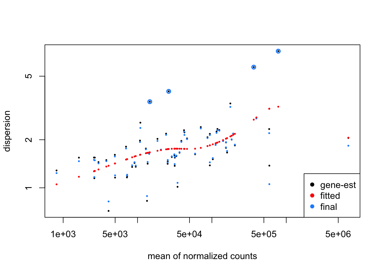
res_zinb <- results(dds_zinb, cooksCutoff = FALSE)
res_zinb
## log2 fold change (MLE): location Kerala vs Bhopal
## LRT p-value: '~ location' vs '~ 1'
## DataFrame with 64 rows and 6 columns
## baseMean log2FoldChange lfcSE stat
## <numeric> <numeric> <numeric> <numeric>
## Megamonas_hypermegale 13681.88 -0.524105 0.331636 0.670188
## Megamonas_funiformis 4956.85 0.535896 0.345018 0.522582
## Megamonas_rupellensis 14621.03 -2.654645 0.512151 4.374362
## Mitsuokella_multacida 115487.83 -0.714622 0.409155 1.036680
## Acidaminococcus_intestini 10919.18 -0.660104 0.423882 0.531985
## ... ... ... ... ...
## Sutterella_wadsworthensis 59450.9 0.9850659 0.352212 3.11392028
## Haemophilus_parainfluenzae 28899.5 -0.3708765 0.345377 0.67126600
## Klebsiella_pneumoniae 193435.7 -0.6070505 0.406656 1.19066189
## Enterobacter_cloacae 31284.0 -0.3529664 0.350424 0.34042735
## Escherichia_coli 396628.7 -0.0474002 0.454280 0.00899331
## pvalue padj
## <numeric> <numeric>
## Megamonas_hypermegale 0.4129862 0.677721
## Megamonas_funiformis 0.4697422 0.715798
## Megamonas_rupellensis 0.0364835 0.179611
## Mitsuokella_multacida 0.3085950 0.580885
## Acidaminococcus_intestini 0.4657737 0.715798
## ... ... ...
## Sutterella_wadsworthensis 0.0776259 0.276003
## Haemophilus_parainfluenzae 0.4126106 0.677721
## Klebsiella_pneumoniae 0.2751961 0.533714
## Enterobacter_cloacae 0.5595827 0.774180
## Escherichia_coli 0.9244474 0.957563df_res_zinb <- cbind(as(res_zinb, "data.frame"), as(tax_table(ps)[rownames(res_zinb), ], "matrix"))
df_res_zinb <- df_res_zinb %>%
rownames_to_column(var = "OTU") %>%
arrange(padj)
fdr_otu_zinb <- df_res_zinb %>%
filter(padj < 0.1) %>%
droplevels() %>%
arrange(desc(padj))
(p2 <- ggplot(fdr_otu_zinb, aes(x = Species, y = log2FoldChange, color = Species)) +
geom_point(size = 4) +
labs(y = "\nLog2 Fold-Change for Kerala vs. Bhopal", x = "") +
theme(axis.text.x = element_text(color = "black", size = 12),
axis.text.y = element_text(color = "black", size = 12),
axis.title.y = element_text(size = 14),
axis.title.x = element_text(size = 14),
legend.text = element_text(size = 12),
legend.title = element_text(size = 12),
legend.position = "none") +
coord_flip() +
geom_hline(yintercept = 0, linetype="dotted"))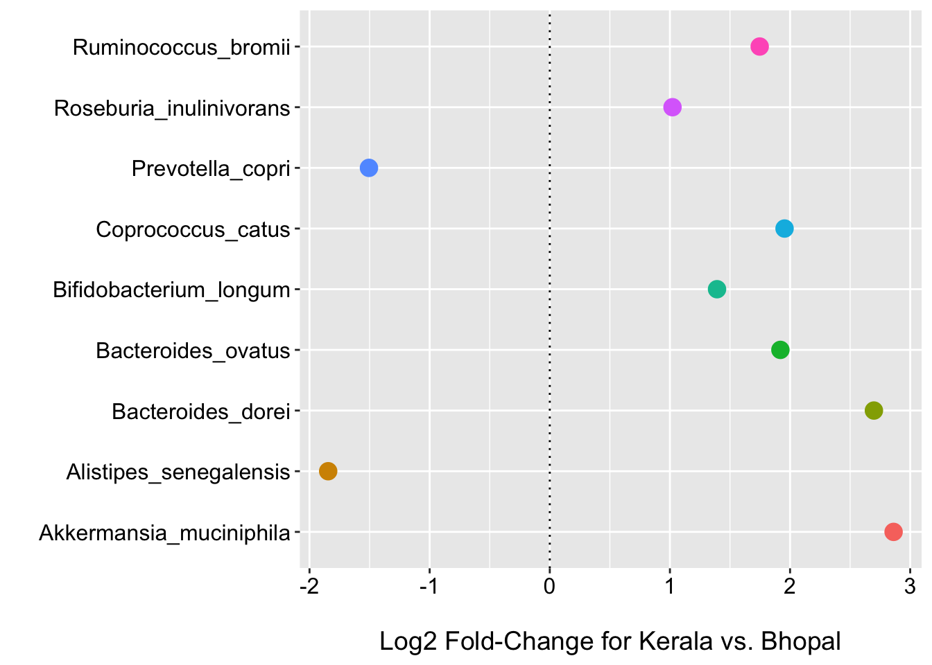
resultsNames(dds_zinb)## [1] "Intercept" "location_Kerala_vs_Bhopal"res_LFC_zinb <- lfcShrink(dds_zinb, coef=2, type="apeglm")## using 'apeglm' for LFC shrinkage. If used in published research, please cite:
## Zhu, A., Ibrahim, J.G., Love, M.I. (2018) Heavy-tailed prior distributions for
## sequence count data: removing the noise and preserving large differences.
## Bioinformatics. https://doi.org/10.1093/bioinformatics/bty895plotMA(res_LFC_zinb)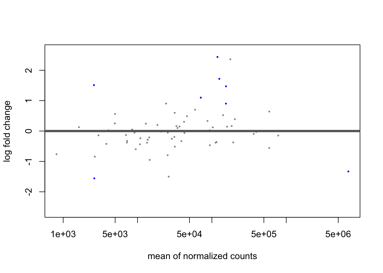
df_res_lfc_zinb <- cbind(as(res_LFC_zinb, "data.frame"), as(tax_table(ps)[rownames(res_LFC_zinb), ], "matrix"))
df_res_lfc_zinb <- df_res_lfc_zinb %>%
  rownames_to_column(var = "OTU") %>%
  arrange(desc(log2FoldChange))

lfc_otu_zinb <- df_res_lfc_zinb %>%
  filter(abs(log2FoldChange) > 1) %>%
  droplevels() %>%
  arrange(desc(log2FoldChange))

(p3 <- ggplot(lfc_otu_zinb, aes(x = Species, y = log2FoldChange, color = Species)) +
  geom_point(size = 4) +
  labs(y = "\nLog2 Fold-Change for Kerala vs. Bhopal", x = "") +
  theme(axis.text.x = element_text(color = "black", size = 12),
        axis.text.y = element_text(color = "black", size = 12),
        axis.title.y = element_text(size = 14),
        axis.title.x = element_text(size = 14),
        legend.text = element_text(size = 12),
        legend.title = element_text(size = 12),
        legend.position = "none") +
  coord_flip() +
  geom_hline(yintercept = 0, linetype="dotted"))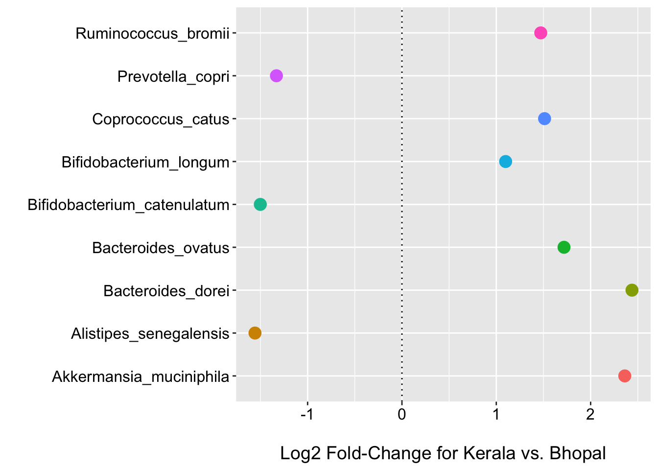
Now we see that 9 species have FDR p-values < 0.1; including R.bromii which had the largest log2 fold-change before. We also see 9 have log2 fold-changes of +/- 1 after shrinkage.
Let’s see if these are the same taxa….
intersect(fdr_otu_zinb$OTU, lfc_otu_zinb$OTU)## [1] "Coprococcus_catus" "Bifidobacterium_longum"
## [3] "Akkermansia_muciniphila" "Ruminococcus_bromii"
## [5] "Alistipes_senegalensis" "Prevotella_copri"
## [7] "Bacteroides_ovatus" "Bacteroides_dorei"zinb_venn <- venn.diagram(
x = list(fdr_otu_zinb$OTU, lfc_otu_zinb$OTU),
category.names = c("ZINB:FDR" , "ZINB:LFC"),
filename = NULL,
fill = c("green", "blue"))
grid::grid.newpage()
grid::grid.draw(zinb_venn) 
cowplot::plot_grid(p2, p3, nrow = 1, ncol = 2, scale = .9, labels = c("FDR", "LFC:apeglm")) 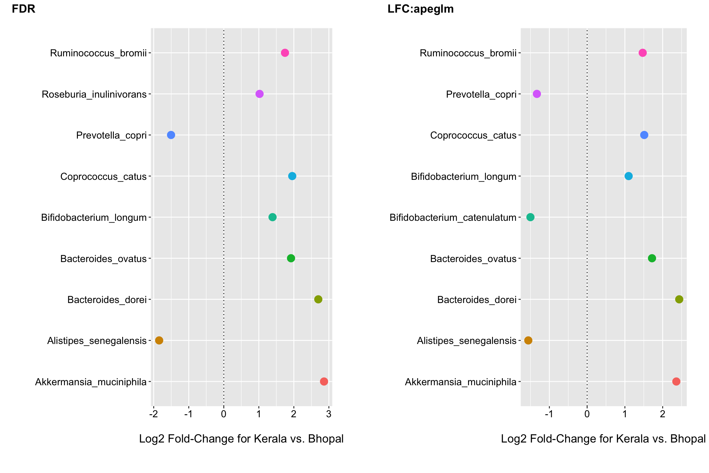 We look to have good overlap and the fold changes for the default and apeglm shrinkage approaches are in good agreement. Next I would look to see if any of the differences were driven by outliers and perhaps consider a few attentive modeling strategies to assess the robustness of the findings before concluding that these species seem to be changing/differing in relative abundance the most between groups.
Concluding remarks
Zero inflated models may better meet the assumed data generating process for some microbiome studies (if we expect that some species simply are not members of some participants microbiota and we would never detect them no matter how deep we were to sequence). Thus, the use of zero-inflation observation weights provides one approach to account for excess zeros when using tools originally designed for bulk RNA-seq. It may also provide for increased statistical power if the weights improve the estimation of the dispersion.
Count-based models like DESeq2 also use normalizations based on log-ratio transforms (i.e., centered log-ratio) and can directly account for excess zeros using mixture models or weights without the need to impute zero values. This makes them attractive alternatives to compositional data analysis approaches when many zeros are present.
The goal of this post is to provide a quick example on how one might go about fitting this type of model to microbiome data. Any thoughts or comments regarding improvements over what is presented here, or advances in this area, are most welcome.
Session Info
sessionInfo()## R version 4.0.2 (2020-06-22)
## Platform: x86_64-apple-darwin17.0 (64-bit)
## Running under: macOS Catalina 10.15.6
##
## Matrix products: default
## BLAS: /Library/Frameworks/R.framework/Versions/4.0/Resources/lib/libRblas.dylib
## LAPACK: /Library/Frameworks/R.framework/Versions/4.0/Resources/lib/libRlapack.dylib
##
## locale:
## [1] en_US.UTF-8/en_US.UTF-8/en_US.UTF-8/C/en_US.UTF-8/en_US.UTF-8
##
## attached base packages:
## [1] grid stats4 parallel stats graphics grDevices utils
## [8] datasets methods base
##
## other attached packages:
## [1] MASS_7.3-51.6 pscl_1.5.5
## [3] VennDiagram_1.6.20 futile.logger_1.4.3
## [5] cowplot_1.1.0 scran_1.16.0
## [7] zinbwave_1.10.1 SingleCellExperiment_1.10.1
## [9] apeglm_1.10.0 DESeq2_1.28.1
## [11] SummarizedExperiment_1.18.2 DelayedArray_0.14.1
## [13] matrixStats_0.56.0 GenomicRanges_1.40.0
## [15] GenomeInfoDb_1.24.2 IRanges_2.22.2
## [17] S4Vectors_0.26.1 phyloseq_1.32.0
## [19] curatedMetagenomicData_1.18.2 ExperimentHub_1.14.2
## [21] Biobase_2.48.0 AnnotationHub_2.20.2
## [23] BiocFileCache_1.12.1 dbplyr_1.4.4
## [25] BiocGenerics_0.34.0 forcats_0.5.0
## [27] stringr_1.4.0 dplyr_1.0.2
## [29] purrr_0.3.4 readr_1.3.1
## [31] tidyr_1.1.2 tibble_3.0.3
## [33] ggplot2_3.3.2 tidyverse_1.3.0
##
## loaded via a namespace (and not attached):
## [1] readxl_1.3.1 backports_1.1.9
## [3] plyr_1.8.6 igraph_1.2.5
## [5] splines_4.0.2 BiocParallel_1.22.0
## [7] scater_1.16.2 digest_0.6.27
## [9] foreach_1.5.0 htmltools_0.5.0
## [11] viridis_0.5.1 fansi_0.4.1
## [13] magrittr_2.0.1 memoise_1.1.0
## [15] cluster_2.1.0 limma_3.44.3
## [17] Biostrings_2.56.0 annotate_1.66.0
## [19] modelr_0.1.8 bdsmatrix_1.3-4
## [21] colorspace_1.4-1 blob_1.2.1
## [23] rvest_0.3.6 rappdirs_0.3.1
## [25] haven_2.3.1 xfun_0.19
## [27] crayon_1.3.4 RCurl_1.98-1.2
## [29] jsonlite_1.7.1 genefilter_1.70.0
## [31] survival_3.1-12 iterators_1.0.12
## [33] ape_5.4-1 glue_1.4.2
## [35] gtable_0.3.0 zlibbioc_1.34.0
## [37] XVector_0.28.0 BiocSingular_1.4.0
## [39] Rhdf5lib_1.10.1 scales_1.1.1
## [41] futile.options_1.0.1 mvtnorm_1.1-1
## [43] edgeR_3.30.3 DBI_1.1.0
## [45] Rcpp_1.0.5 viridisLite_0.3.0
## [47] xtable_1.8-4 emdbook_1.3.12
## [49] dqrng_0.2.1 rsvd_1.0.3
## [51] bit_4.0.4 httr_1.4.2
## [53] RColorBrewer_1.1-2 ellipsis_0.3.1
## [55] farver_2.0.3 pkgconfig_2.0.3
## [57] XML_3.99-0.5 locfit_1.5-9.4
## [59] labeling_0.3 softImpute_1.4
## [61] tidyselect_1.1.0 rlang_0.4.8
## [63] reshape2_1.4.4 later_1.1.0.1
## [65] AnnotationDbi_1.50.3 munsell_0.5.0
## [67] BiocVersion_3.11.1 cellranger_1.1.0
## [69] tools_4.0.2 cli_2.0.2
## [71] generics_0.0.2 RSQLite_2.2.0
## [73] ade4_1.7-15 broom_0.7.0
## [75] evaluate_0.14 biomformat_1.16.0
## [77] fastmap_1.0.1 yaml_2.2.1
## [79] knitr_1.30 bit64_4.0.5
## [81] fs_1.5.0 nlme_3.1-148
## [83] mime_0.9 formatR_1.7
## [85] xml2_1.3.2 compiler_4.0.2
## [87] rstudioapi_0.11 beeswarm_0.2.3
## [89] curl_4.3 interactiveDisplayBase_1.26.3
## [91] reprex_0.3.0 statmod_1.4.34
## [93] geneplotter_1.66.0 stringi_1.5.3
## [95] blogdown_0.21.45 lattice_0.20-41
## [97] Matrix_1.2-18 vegan_2.5-6
## [99] permute_0.9-5 multtest_2.44.0
## [101] vctrs_0.3.4 pillar_1.4.6
## [103] lifecycle_0.2.0 BiocManager_1.30.10
## [105] BiocNeighbors_1.6.0 irlba_2.3.3
## [107] data.table_1.13.0 bitops_1.0-6
## [109] httpuv_1.5.4 R6_2.5.0
## [111] bookdown_0.21 promises_1.1.1
## [113] gridExtra_2.3 vipor_0.4.5
## [115] codetools_0.2-16 lambda.r_1.2.4
## [117] assertthat_0.2.1 rhdf5_2.32.2
## [119] withr_2.2.0 GenomeInfoDbData_1.2.3
## [121] mgcv_1.8-31 hms_0.5.3
## [123] coda_0.19-4 DelayedMatrixStats_1.10.1
## [125] rmarkdown_2.5 bbmle_1.0.23.1
## [127] numDeriv_2016.8-1.1 shiny_1.5.0
## [129] lubridate_1.7.9 ggbeeswarm_0.6.0