Introduction to the Statistical Analysis of Microbiome Data in R
This post is also from the Introduction to Metagenomics Summer Workshop and provides a quick introduction to some common analytic methods used to analyze microbiome data. I thought it might be of interest to a broader audience so decided to post it here.
The goal of this session is to provide you with a high-level introduction to some common analytic methods used to analyze microbiome data. It will also serve to introduce you several popular R packages developed specifically for microbiome data analysis. We chose to emphasize R for this course because of the rapid development of methods and packages provided in the R language, the breadth of existing tutorials and resources, and the ever expanding community of R users. However, other platforms such as QIIME2, biobakery and USEARCH, just to name a few, offer excellent integrated solutions for the processing and analysis of amplicon and/or shotgun metagenomic sequence data.
The diverse goals and technical variation of metagenomic research projects does not allow for a standard “analytic pipeline” for microbiome data analysis. Approaching the analysis of microbiome data with a single workflow in mind is generally not a great idea, as there is no “one size fits all” solution for the assorted set of questions one might want to answer. However, you may be surprised to find that projects on very different topics often have overarching analytic aims such as:
- Describing the microbial community composition of a set of samples
- Estimating within- and between-sample diversity
- Identifying differentially abundant taxa
- Predicting a response from a set of taxonomic features
- Assessing microbial network structures and patterns of co-occurance
- Exploring the phylogenetic relatedness of a set of organisms
We will cover statistical methods developed to address several of these aims with a focus on introducing you to their implementation in R. A detailed description of each approach, its assumptions, package options, etc. is beyond the scope of this session. However, I try to provide links to source materials and more detailed documentation where possible. The statistical analysis of microbial metagenomic sequence data is a rapidly evolving field and different solutions (often many) have been proposed to answer the same questions. I have tried to focus on methods that are common in the microbiome literature, well-documented, and reasonably accessible…and a few I think are new and interesting. I also try to show a few different approaches in each section. In cases where I focus largely on more basic implementations, I have tried to provide links for advanced learning of more complex topics.
The publicly available data used in this session are from Giloteaux et. al. Reduced diversity and altered composition of the gut microbiome in individuals with myalgic encephalomyelitis/chronic fatigue syndrome published in Microbiome (2016). The metadata, OTU table, and taxonomy files were obtained from the QIIME2 tutorial Differential abundance analysis with gneiss (accessed on 06/13/2019). The code and data used to generate the phyloseq object is provided on my GitHub page. The data were generated by 16S rRNA gene sequencing (V4 hypervariable region) of fecal samples on the Illumina MiSeq. Our focus will be on examining differences in the microbiota of patients with chronic fatigue syndrome versus healthy controls. We will examine:
- Taxonomic relative abundance
- Hierarchal clustering
- Alpha-diversity
- Beta-diversity
- Differential abundance testing
- Predicting class labels
Additional resources
There are many great resources for conducting microbiome data analysis in R. Statistical Analysis of Microbiome Data in R by Xia, Sun, and Chen (2018) is an excellent textbook in this area. For those looking for an end-to-end workflow for amplicon data in R, I highly recommend Ben Callahan’s F1000 Research paper Bioconductor Workflow for Microbiome Data Analysis: from raw reads to community analyses. In addition there are numerous websites and vignettes dedicated to microbiome analyses. A few include:
- Paul McMurdie’s phyloseq website
- Robert Edgar’s website
- The microbiome R package website
- All the materials and resources posted on the STAMPS wiki page (a course I highly recommend!)
Installing packages
The code below will install the packages needed to run the analyses. These packages are installed from CRAN, Bioconductor and from developer GitHub sites. Several of these packages are large, and have many dependencies, so this will take some time. This code was modified from Ben’s Bioconductor paper.
In general, package management and versioning can be a challenge for those new to R. Inevitably, if you do not take steps ahead of time, you will find that one of your programs that ran fine just a few months ago, no longer works! Often this is because changes in new versions of packages or R caused your code to break. There are multiple solutions depending on your goals, and all come with pros and cons, but a good place to start is to learn more about Packrat and other package management tools.
If you already have many/some of these packages installed on your local system, you may want to skip this step and install manually only those that you need.
.cran_packages <- c("tidyverse", "cowplot", "picante", "vegan", "HMP", "dendextend", "rms", "devtools")
.bioc_packages <- c("phyloseq", "DESeq2", "microbiome", "metagenomeSeq", "ALDEx2")
.inst <- .cran_packages %in% installed.packages()
if(any(!.inst)) {
  install.packages(.cran_packages[!.inst])
}
if (!requireNamespace("BiocManager", quietly = TRUE))
  install.packages("BiocManager")
BiocManager::install(.bioc_packages, version = "3.9")
devtools::install_github("adw96/breakaway")
devtools::install_github(repo = "UVic-omics/selbal")
Loading required packages
Let’s load the required packages. This is not the most elegant way to do this, but it allows you to see each package that is loaded and the version number.
library(tidyverse); packageVersion("tidyverse") ## [1] '1.3.0'library(phyloseq); packageVersion("phyloseq") ## [1] '1.32.0'library(DESeq2); packageVersion("DESeq2") ## [1] '1.28.1'library(microbiome); packageVersion("microbiome") ## [1] '1.10.0'library(vegan); packageVersion("vegan") ## [1] '2.5.6'library(picante); packageVersion("picante") ## [1] '1.8.2'library(ALDEx2); packageVersion("ALDEx2") ## [1] '1.21.1'library(metagenomeSeq); packageVersion("metagenomeSeq") ## [1] '1.30.0'library(HMP); packageVersion("HMP") ## [1] '2.0.1'library(dendextend); packageVersion("dendextend") ## [1] '1.14.0'library(selbal); packageVersion("selbal") ## [1] '0.1.0'library(rms); packageVersion("rms")## [1] '6.0.1'library(breakaway); packageVersion("breakaway") ## [1] '4.7.2'Reading in the Giloteaux data
The data from the Giloteaux et. al. 2016 paper has been saved as a phyloseq object. We will use the readRDS() function to read it into R. We will also examine the distribution of read counts (per sample library size/read depth/total reads) and remove samples with < 5k total reads. We will then create a new metadata field “Status” that provides more “descriptive” values for our primary variable of interest; whether or not the sample was from a patient with chronic fatigue syndrome or a healthy control.
This should all be familiar to those of you who worked through the Introduction to Phyloseq session. However, something that will be new is that now we are using pipes from the magrittr package and tidyverse verbs to streamline some of the data manipulation steps. For those of you have not worked with the tidyverse set of packages and functions you are missing out! They will change they way you work in R. R for Data Science is an excellent source to learn more about the tidyverse packages and philosophy for data science.
Additional quality controls checks and data pre-processing specific to the goals of your project should be conducted at this point (but is outside of the scope of the current session).
#Read in ps object
(ps <- readRDS("/Users/olljt2/Desktop/hugo_blog/static/data/ps_giloteaux_2016.rds"))
## phyloseq-class experiment-level object
## otu_table() OTU Table: [ 138 taxa and 87 samples ]
## sample_data() Sample Data: [ 87 samples by 22 sample variables ]
## tax_table() Taxonomy Table: [ 138 taxa by 7 taxonomic ranks ]
## phy_tree() Phylogenetic Tree: [ 138 tips and 137 internal nodes ]
## refseq() DNAStringSet: [ 138 reference sequences ]#Sort samples on total read count, remove <5k reads, remove any OTUs seen in only those samples
sort(phyloseq::sample_sums(ps)) ## ERR1331827 ERR1331852 ERR1331856 ERR1331869 ERR1331833 ERR1331797 ERR1331786
## 2707 3031 3117 5083 5245 5307 5696
## ERR1331818 ERR1331792 ERR1331803 ERR1331793 ERR1331819 ERR1331858 ERR1331807
## 5733 6463 6512 6622 6900 6913 7121
## ERR1331815 ERR1331821 ERR1331843 ERR1331795 ERR1331846 ERR1331811 ERR1331845
## 7179 7272 7284 7314 7569 7665 7815
## ERR1331842 ERR1331838 ERR1331855 ERR1331824 ERR1331832 ERR1331804 ERR1331868
## 7911 8102 8115 8148 8186 8236 8612
## ERR1331831 ERR1331859 ERR1331790 ERR1331789 ERR1331837 ERR1331857 ERR1331801
## 8840 9016 9085 9184 9731 9966 11173
## ERR1331841 ERR1331861 ERR1331820 ERR1331854 ERR1331863 ERR1331806 ERR1331787
## 11442 11826 12940 13029 13094 13095 13690
## ERR1331853 ERR1331851 ERR1331836 ERR1331835 ERR1331802 ERR1331799 ERR1331847
## 14113 14365 14488 14753 14799 14833 15290
## ERR1331834 ERR1331817 ERR1331809 ERR1331828 ERR1331813 ERR1331798 ERR1331816
## 15367 15460 16162 16494 16749 16947 17015
## ERR1331830 ERR1331785 ERR1331823 ERR1331865 ERR1331848 ERR1331800 ERR1331867
## 17457 17557 18506 19013 19257 19443 19732
## ERR1331870 ERR1331810 ERR1331825 ERR1331866 ERR1331871 ERR1331849 ERR1331860
## 19783 19909 20069 20760 20862 21540 21553
## ERR1331808 ERR1331872 ERR1331812 ERR1331850 ERR1331791 ERR1331788 ERR1331796
## 21713 22339 22518 22639 23246 23751 23792
## ERR1331840 ERR1331826 ERR1331822 ERR1331862 ERR1331864 ERR1331829 ERR1331844
## 24752 28186 28556 31064 44533 51918 57214
## ERR1331805 ERR1331839 ERR1331794
## 59355 61206 65941(ps <- phyloseq::subset_samples(ps, phyloseq::sample_sums(ps) > 5000)) ## phyloseq-class experiment-level object
## otu_table() OTU Table: [ 138 taxa and 84 samples ]
## sample_data() Sample Data: [ 84 samples by 22 sample variables ]
## tax_table() Taxonomy Table: [ 138 taxa by 7 taxonomic ranks ]
## phy_tree() Phylogenetic Tree: [ 138 tips and 137 internal nodes ]
## refseq() DNAStringSet: [ 138 reference sequences ](ps <- phyloseq::prune_taxa(phyloseq::taxa_sums(ps) > 0, ps)) ## phyloseq-class experiment-level object
## otu_table() OTU Table: [ 138 taxa and 84 samples ]
## sample_data() Sample Data: [ 84 samples by 22 sample variables ]
## tax_table() Taxonomy Table: [ 138 taxa by 7 taxonomic ranks ]
## phy_tree() Phylogenetic Tree: [ 138 tips and 137 internal nodes ]
## refseq() DNAStringSet: [ 138 reference sequences ]#Assign new sample metadata field
phyloseq::sample_data(ps)$Status <- ifelse(phyloseq::sample_data(ps)$Subject == "Patient", "Chronic Fatigue", "Control")
phyloseq::sample_data(ps)$Status <- factor(phyloseq::sample_data(ps)$Status, levels = c("Control", "Chronic Fatigue"))
ps %>%
sample_data %>%
dplyr::count(Status)## Warning in class(x) <- c(setdiff(subclass, tibble_class), tibble_class): Setting
## class(x) to multiple strings ("tbl_df", "tbl", ...); result will no longer be an
## S4 object## Warning in class(x) <- c(setdiff(subclass, tibble_class), tibble_class): Setting
## class(x) to multiple strings ("grouped_df", "tbl_df", ...); result will no
## longer be an S4 object## $Status
## [1] Control Chronic Fatigue
## Levels: Control Chronic Fatigue
##
## $n
## [1] 37 47
##
## attr(,"row.names")
## [1] 1 2
## attr(,"class")
## [1] "sample_data"
## attr(,"class")attr(,"package")
## [1] "phyloseq"
## attr(,".S3Class")
## [1] "data.frame"We can see that we have a phyloseq object consisting of 138 taxa on 84 samples, 22 sample metadata fields, 7 taxonomic ranks and that a phylogenetic tree and the reference sequences have been included. We also see that there are data on n=37 controls and n=47 patients with chronic fatigue.
Visualizing relative abundance
Often an early step in many microbiome projects to visualize the relative abundance of organisms at specific taxonomic ranks. Stacked bar plots and faceted box plots are two ways of doing this. I recommend that if using bar plots to include each sample as a separate observation (and not to aggregate by groups). This is because the sample-to-sample variability can be high, even within groups, which may be just or more important to observe than between-group differences…which can be obscured with aggregation.
The ability to discriminate between more than say a dozen colors in a single plot is also a limitation of the stacked bar plot (faceted box plots do not suffer this limitation). Thus, this is one analysis I often run in QIIME2 using the taxa barplot command, as it allows for beautiful interactive viewing. This could also be done in R using a shiny app. I just haven’t implemented, or seen others implement, this functionality yet in R (I imagine someone has so please let me know if/when you do).
Here we will agglomerate the reads to the phylum-level using phyloseq and plot the relative abundance by Status.
#Get count of phyla
table(phyloseq::tax_table(ps)[, "Phylum"])
##
## Actinobacteria Bacteroidetes Cyanobacteria Euryarchaeota Firmicutes
## 7 11 2 1 105
## Fusobacteria Proteobacteria Tenericutes Verrucomicrobia
## 1 7 2 1#Convert to relative abundance
ps_rel_abund = phyloseq::transform_sample_counts(ps, function(x){x / sum(x)})
phyloseq::otu_table(ps)[1:5, 1:5]## OTU Table: [5 taxa and 5 samples]
## taxa are rows
## ERR1331793 ERR1331872 ERR1331819 ERR1331794 ERR1331851
## OTU1 2 581 347 916 10498
## OTU2 371 46 0 233 301
## OTU3 1189 81 637 199 0
## OTU4 0 172 246 0 372
## OTU5 308 44 143 155 221phyloseq::otu_table(ps_rel_abund)[1:5, 1:5]## OTU Table: [5 taxa and 5 samples]
## taxa are rows
## ERR1331793 ERR1331872 ERR1331819 ERR1331794 ERR1331851
## OTU1 0.0003020236 0.026008326 0.05028986 0.013891206 0.73080404
## OTU2 0.0560253700 0.002059179 0.00000000 0.003533462 0.02095371
## OTU3 0.1795530051 0.003625946 0.09231884 0.003017849 0.00000000
## OTU4 0.0000000000 0.007699539 0.03565217 0.000000000 0.02589628
## OTU5 0.0465116279 0.001969649 0.02072464 0.002350586 0.01538462#Plot
phyloseq::plot_bar(ps_rel_abund, fill = "Phylum") +
geom_bar(aes(color = Phylum, fill = Phylum), stat = "identity", position = "stack") +
labs(x = "", y = "Relative Abundance\n") +
facet_wrap(~ Status, scales = "free") +
theme(panel.background = element_blank(),
axis.text.x=element_blank(),
axis.ticks.x=element_blank())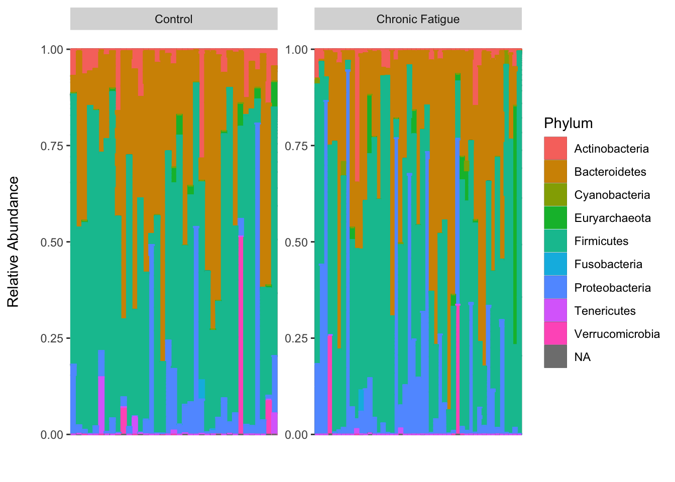
There are a total of nine phyla and their relative abundance looks to be quite simialr between groups. You could sort the taxa on abundance to improve the vizualization. I’ll let you give that a shot on your own. Let’s generate box plots according to group and facet them by phylum using the raw counts. We will use the phyloseq::melt function to help.
#Agglomerate to phylum-level and rename
ps_phylum <- phyloseq::tax_glom(ps, "Phylum")
phyloseq::taxa_names(ps_phylum) <- phyloseq::tax_table(ps_phylum)[, "Phylum"]
phyloseq::otu_table(ps_phylum)[1:5, 1:5]
## OTU Table: [5 taxa and 5 samples]
## taxa are rows
## ERR1331793 ERR1331872 ERR1331819 ERR1331794 ERR1331851
## Bacteroidetes 1903 878 1837 1969 11776
## Proteobacteria 119 3315 468 62358 319
## Firmicutes 4319 14429 3548 1609 2207
## Actinobacteria 30 976 17 0 58
## Cyanobacteria 246 0 0 0 0#Melt and plot
phyloseq::psmelt(ps_phylum) %>%
ggplot(data = ., aes(x = Status, y = Abundance)) +
geom_boxplot(outlier.shape = NA) +
geom_jitter(aes(color = OTU), height = 0, width = .2) +
labs(x = "", y = "Abundance\n") +
facet_wrap(~ OTU, scales = "free")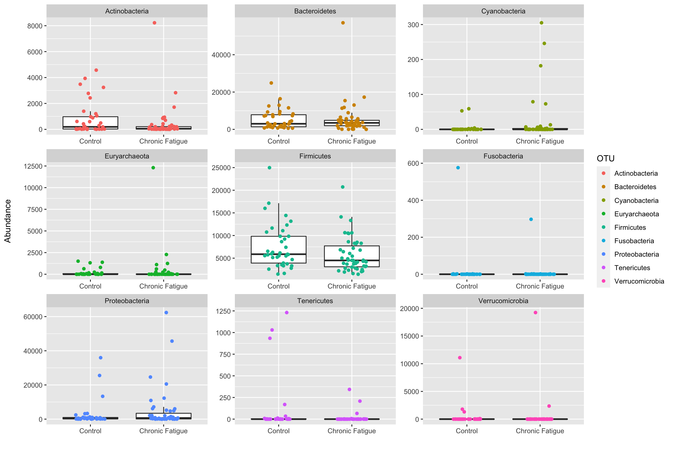
As we saw before, many samples have a high number of Firmicutes, followed by Bacteroidetes, and Actinobacteria. Most samples have low read counts for other phyla with some outlying samples. There does not appear to be much difference in the major phyla between groups. Check out Ben Callahan’s F1000 paper for additional examples on visualizing sequence variant prevalence/abundance that may be helpful for specific analyses.
One way to formally test for a difference in the phylum-level abundance is to conduct a multivariate test for differences in the overall composition between groups of samples. This type of test can be implemented using the HMP package (Xdc.sevsample function) described in the paper Hypothesis Testing and Power Calculations for Taxonomic-Based Human Microbiome Data by La Rosa et. al.
Basically, a Dirichlet-Multinomial distribution is assumed for the data and null hypothesis testing is conducted by testing for a difference in the location (mean distribution of each taxa) across groups accounting for the overdispersion in the count data. The authors describe this test as analogous to a two sample t-test, but instead we are evaluating whether taxa frequencies observed in both groups of metagenomic samples are equal (null hypothesis). Here we are performing the test on bacterial phyla, but it could be performed at any taxonomic level including OTUs. The authors recommend that rare taxa be pooled into a single group to improve testing.
#Subset groups
controls <- phyloseq::subset_samples(ps_phylum, Status == "Control")
cf <- phyloseq::subset_samples(ps_phylum, Status == "Chronic Fatigue")
#Output OTU tables
control_otu <- data.frame(phyloseq::otu_table(controls))
cf_otu <- data.frame(phyloseq::otu_table(cf))
#Group rare phyla
control_otu <- control_otu %>%
  t(.) %>%
  as.data.frame(.) %>%
  mutate(Other = Cyanobacteria + Euryarchaeota + Tenericutes + Verrucomicrobia + Fusobacteria) %>%
  dplyr::select(-Cyanobacteria, -Euryarchaeota, -Tenericutes, -Verrucomicrobia, -Fusobacteria)
cf_otu <- cf_otu %>%
  t(.) %>%
  as.data.frame(.) %>%
  mutate(Other = Cyanobacteria + Euryarchaeota + Tenericutes + Verrucomicrobia + Fusobacteria) %>%
  dplyr::select(-Cyanobacteria, -Euryarchaeota, -Tenericutes, -Verrucomicrobia, -Fusobacteria)
#HMP test
group_data <- list(control_otu, cf_otu)
(xdc <- HMP::Xdc.sevsample(group_data))
## $`Xdc statistics`
## [1] 0.2769004
##
## $`p value`
## [1] 0.99805511 - pchisq(.2769004, 5)## [1] 0.9980551The HMP test fails to reject the null hypothesis of no difference in the distribution of phyla between groups (in line with our expectations). The xdc test follows a Chi-square distribution with degrees of freedom equal to (J-1)*K, where J is the number of groups and K is the number of taxa. The last calculation just shows how the p-value is obtained. The test can be expanded to more than two groups and to test for differences in rank abundance distributions (RAD). These are topics I encourage you to explore on your own. The microbiome package also has some nice functions for visualizing community composition you should look into.
Hierarchical clustering
Another early step in many microbiome projects to examine how samples cluster on some measure of taxonomic (dis)similarity. There are MANY ways to do perform such clustering. Here I present just one approach that I assume many of you are familiar with. We will perform hierarchal clustering of samples based on their Bray-Curtis dissimilarity. Here is a link to how it is calculated. We will discuss this in more detail during the lecture, but for now it should suffice to know that the as two samples share fewer taxa, the number increases. The Bray-Curtis dissimilarity is zero for samples that have the exact same composition and one for those sharing no taxa. It is also worth remembering that this is a measure of dissimilarity (it is not a true distance measure).
We will use the popular vegan package for community ecology to compute the Bray-Curtis dissimilarity for all samples. Then we will apply Ward’s clustering and color code the sample names to assess the extent to which the samples from the control and chronic fatigue participants cluster. At a high-level, Ward’s clustering finds the pair of clusters at each iteration that minimalizes the increase in total variance.
Let’s see how this is done in R.
#Extract OTU table and compute BC
ps_rel_otu <- data.frame(phyloseq::otu_table(ps_rel_abund))
ps_rel_otu <- t(ps_rel_otu)
bc_dist <- vegan::vegdist(ps_rel_otu, method = "bray")
as.matrix(bc_dist)[1:5, 1:5]
## ERR1331793 ERR1331872 ERR1331819 ERR1331794 ERR1331851
## ERR1331793 0.0000000 0.8801040 0.5975550 0.9767218 0.8684629
## ERR1331872 0.8801040 0.0000000 0.7590766 0.9596181 0.9206484
## ERR1331819 0.5975550 0.7590766 0.0000000 0.9556656 0.7810736
## ERR1331794 0.9767218 0.9596181 0.9556656 0.0000000 0.9693291
## ERR1331851 0.8684629 0.9206484 0.7810736 0.9693291 0.0000000#Save as dendrogram
ward <- as.dendrogram(hclust(bc_dist, method = "ward.D2"))
#Provide color codes
meta <- data.frame(phyloseq::sample_data(ps_rel_abund))
colorCode <- c(Control = "red", `Chronic Fatigue` = "blue")
labels_colors(ward) <- colorCode[meta$Status][order.dendrogram(ward)]
#Plot
plot(ward)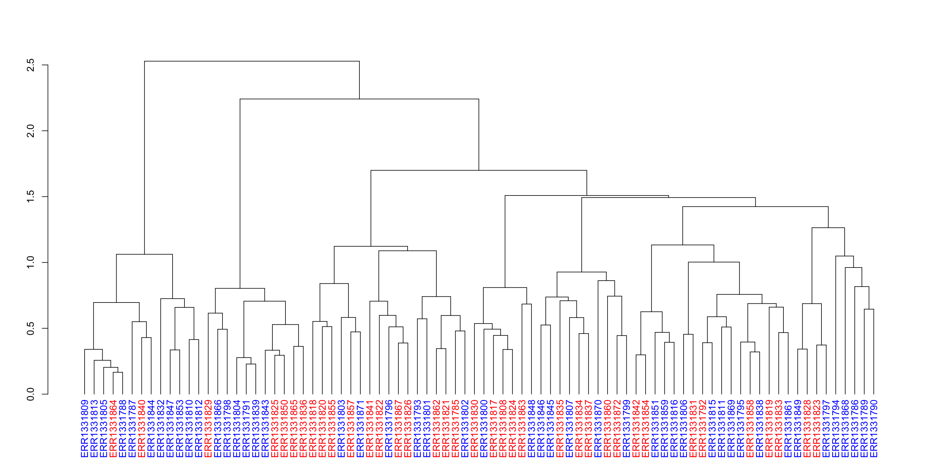
We can see that the Bray-Curtis dissimilarity for these selected samples range from around 0.6 to close to 1. Thus, the composition of some samples are quite different from one another. We also see some clustering according to Status near the tips, but no clear “higher-level” clustering. We will try to exploit this information later to see if we can predict the label of each sample with only information on the microbial relative abundances.
Heatmaps are another good way to visualize these types of associations and can be implemented using phyloseq. Give it a try on your own!
Alpha-diversity
Robert Edgar provides an excellent definition of alpha-diversity on his website:
Alpha-diversity is the diversity in a single ecosystem or sample. The simplest measure is richness, the number of species (or OTUs) observed in the sample. Other metrics consider the abundances (frequencies) of the OTUs, for example to give lower weight to lower-abundance OTUs.
Basically, it is the within-sample diversity and includes how many organisms are observed (i.e. observed OTUs) and how evenly they are distributed. Many researchers are interested in estimating alpha-diversity since differences between groups have been associated with several health related outcomes. However the issue of how to best estimate these quantities using data derived from next-generation sequencing (NGS) is controversial. This is due to two main reasons:
- The observed richness in a sample/site is typically underestimated due to inexhaustive sampling. Thus, valid estimators of diversity require extrapolating from the available observations to provide estimates of the unobserved taxa (and also account for the sampling variability).
- Extrapolation estimators require an accurate count of the rare taxa (including singletons) in each sample…which for NGS-based metagenomics studies we typically do not have…since singletons generally cannot be differentiated from sequencing errors using the current best informatics workflows. The extent to which we cannot accurately detect low abundance taxa limits the utility of diversity estimators reliant upon such counts.
So we are kind of in a catch-22 regarding the best way forward given current technologies.
It has been argued; however, that diversity metrics can nevertheless be compared between samples because the errors and biases are mostly systematic (i.e. occur with similar rates in all samples). See Dr. Edgar’s discussion of the topic here for more detail. This is what is typically done in most published studies to date. A major underlying assumption here is that abundance structures are the same for the two groups being compared. This is perhaps a reasonable assumption when comparing similar environments, but it is hard to know without exhaustive sampling. See figure 1 here and the related discussion by Amy Willis for a more detailed understanding of how the abundance structure can lead you to incorrect conclusions (quite disconcerting).
Rarefaction (subsampling reads from each sample without replacement to a constant depth) is often performed before estimating alpha-diversity; although, it is unclear to me if/when this helps since environments can be identical with respect to one alpha diversity metric, but the different abundance structures will induce different biases when rarified (italicized text taken from Amy’s paper linked to above).
Dr. Willis has examined this issue in depth and developed breakaway and DivNet to specifically address the shortcoming of current approaches. I highly recommend you check out her GitHub site. In a recent paper she argues:
In order to draw meaningful conclusions about the entire microbial community, it is necessary to adjust for inexhaustive sampling using statistically-motivated parameter estimates for alpha diversity. In order to draw meaningful conclusions regarding comparisons of microbial communities, it is necessary to use measurement error models to adjust for the uncertainty in the estimation of alpha diversity. She also states that breakaway is not overly sensitive to singleton counts.
The links below provide a brief introduction to the topic. I look forward to Amy’s updated tutorial and thoughts on when microbial diversity estimation is, and isn’t, possible as mentioned in the last link (I suspect it will result in some updating of these materials).
- https://www.drive5.com/usearch/manual/alpha_diversity.html
- https://www.biorxiv.org/content/biorxiv/early/2017/12/11/231878.full.pdf
- https://github.com/benjjneb/dada2/issues/103
- https://github.com/benjjneb/dada2/issues/317
Below we will estimate and test for differences according to chronic fatigue status using the plug-in estimates for observed richness, Shannon diversity, and phylogenetic diversity on the subsampled data (since this is common practice). I have also provided some code to estimate richness using breakaway that you can examine on your own. I plan to update this section with some data that is more appropriate for breakaway. So check back soon.
ggplot(data = data.frame("total_reads" =  phyloseq::sample_sums(ps),
                         "observed" = phyloseq::estimate_richness(ps, measures = "Observed")[, 1]),
       aes(x = total_reads, y = observed)) +
  geom_point() +
  geom_smooth(method="lm", se = FALSE) +
  labs(x = "\nTotal Reads", y = "Observed Richness\n")
## `geom_smooth()` using formula 'y ~ x'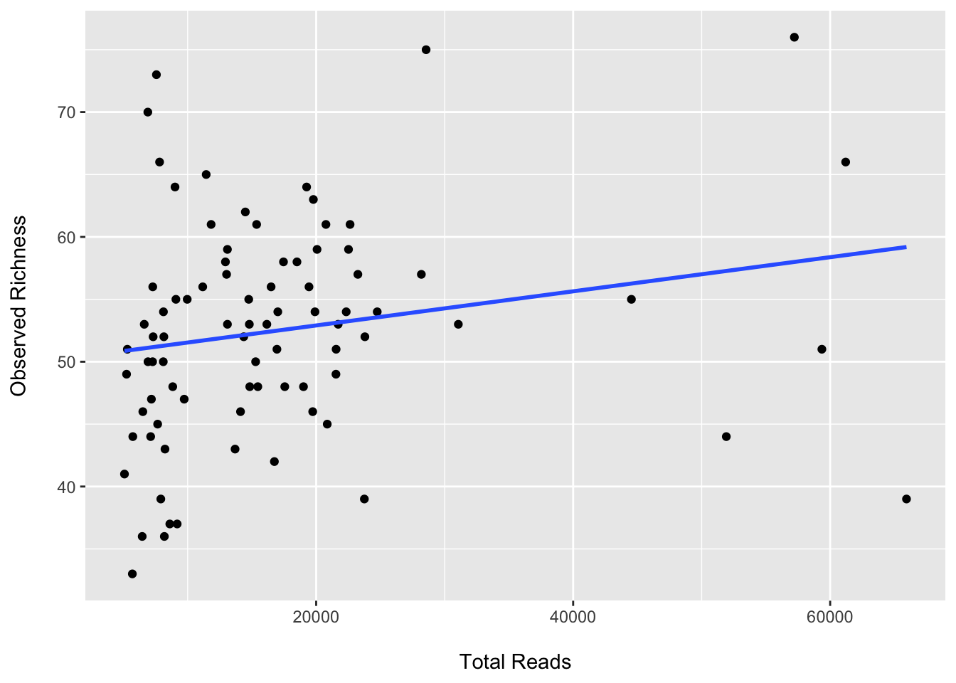
We see that the observed OTUs are correlated with the total read count (as expected). Now let’s subsample, plot, and test for group differences.
#Subsample reads
(ps_rare <- phyloseq::rarefy_even_depth(ps, rngseed = 123, replace = FALSE))
## `set.seed(123)` was used to initialize repeatable random subsampling.## Please record this for your records so others can reproduce.## Try `set.seed(123); .Random.seed` for the full vector## ...## phyloseq-class experiment-level object
## otu_table() OTU Table: [ 138 taxa and 84 samples ]
## sample_data() Sample Data: [ 84 samples by 23 sample variables ]
## tax_table() Taxonomy Table: [ 138 taxa by 7 taxonomic ranks ]
## phy_tree() Phylogenetic Tree: [ 138 tips and 137 internal nodes ]
## refseq() DNAStringSet: [ 138 reference sequences ]head(phyloseq::sample_sums(ps_rare))## ERR1331793 ERR1331872 ERR1331819 ERR1331794 ERR1331851 ERR1331834
## 5083 5083 5083 5083 5083 5083#Generate a data.frame with adiv measures
adiv <- data.frame(
"Observed" = phyloseq::estimate_richness(ps_rare, measures = "Observed"),
"Shannon" = phyloseq::estimate_richness(ps_rare, measures = "Shannon"),
"PD" = picante::pd(samp = data.frame(t(data.frame(phyloseq::otu_table(ps_rare)))), tree = phyloseq::phy_tree(ps_rare))[, 1],
"Status" = phyloseq::sample_data(ps_rare)$Status)
head(adiv)## Observed Shannon PD Status
## ERR1331793 53 2.7462377 20.597980 Chronic Fatigue
## ERR1331872 52 2.7527053 21.289719 Control
## ERR1331819 70 3.2378006 21.671340 Control
## ERR1331794 27 0.3761523 8.275154 Chronic Fatigue
## ERR1331851 45 1.3387308 14.783592 Chronic Fatigue
## ERR1331834 54 2.8883445 20.988640 Control#Plot adiv measures
adiv %>%
gather(key = metric, value = value, c("Observed", "Shannon", "PD")) %>%
mutate(metric = factor(metric, levels = c("Observed", "Shannon", "PD"))) %>%
ggplot(aes(x = Status, y = value)) +
geom_boxplot(outlier.color = NA) +
geom_jitter(aes(color = Status), height = 0, width = .2) +
labs(x = "", y = "") +
facet_wrap(~ metric, scales = "free") +
theme(legend.position="none")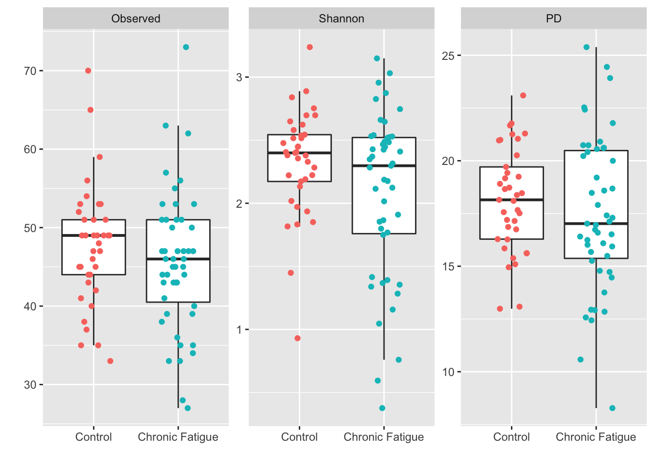
#Summarize
adiv %>%
  group_by(Status) %>%
  dplyr::summarise(median_observed = median(Observed),
            median_shannon = median(Shannon),
            median_pd = median(PD))
## `summarise()` ungrouping output (override with `.groups` argument)## # A tibble: 2 x 4
## Status median_observed median_shannon median_pd
## <fct> <dbl> <dbl> <dbl>
## 1 Control 49 2.40 18.1
## 2 Chronic Fatigue 46 2.30 17.0#Wilcoxon test of location
wilcox.test(Observed ~ Status, data = adiv, exact = FALSE, conf.int = TRUE)##
## Wilcoxon rank sum test with continuity correction
##
## data: Observed by Status
## W = 1007.5, p-value = 0.2146
## alternative hypothesis: true location shift is not equal to 0
## 95 percent confidence interval:
## -1.000059 5.000002
## sample estimates:
## difference in location
## 2.000087wilcox.test(Shannon ~ Status, data = adiv, conf.int = TRUE) ##
## Wilcoxon rank sum exact test
##
## data: Shannon by Status
## W = 1037, p-value = 0.1329
## alternative hypothesis: true location shift is not equal to 0
## 95 percent confidence interval:
## -0.04346366 0.39218192
## sample estimates:
## difference in location
## 0.1421467wilcox.test(PD ~ Status, data = adiv, conf.int = TRUE)##
## Wilcoxon rank sum exact test
##
## data: PD by Status
## W = 995, p-value = 0.2616
## alternative hypothesis: true location shift is not equal to 0
## 95 percent confidence interval:
## -0.7452342 2.1356893
## sample estimates:
## difference in location
## 0.6854015Here we see a modestly lower median alpha-diversity in samples from participants with chronic fatigue when compared to healthy controls. However, the variation in alpha-diversity between groups is highly overlapping and we fail to reject the null hypothesis of no difference in location between groups.
Below is the code to estimate richness using breakaway. You will see some warnings. I plan to update this section with some additional data so check back soon.
#Obtain breakaway estimates
ba_adiv <- breakaway::breakaway(ps)
ba_adiv[1]
#Plot estimates
plot(ba_adiv, ps, color = "Status")
#Examine models
summary(ba_adiv) %>%
  add_column("SampleNames" = ps %>% otu_table %>% sample_names)
#Test for group differnce
bt <- breakaway::betta(summary(ba_adiv)$estimate,
                       summary(ba_adiv)$error,
                       make_design_matrix(ps, "Status"))
bt$table
Beta-diversity
Beta-diversity provides a measure of similarity, or dissimilarity, of one microbial composition to another. Beta-diversity is typically calculated on the OTU/ASV/species composition tables directly (after normalization), but can be calculated using abundances at higher taxonomic levels. One common estimator of microbial beta-diversity is the pairwise Euclidean distance between samples. However, many ecologically informative measures are also commonly used and include:
- Bray-Curtis similarity
- Jaccard similarity
- Yue & Clayton theta similarity
- UniFrac distance
- AND MANY MORE
Pat Schloss provides a listing and links to a large number of alpha- and beta-diversity estimators on his mothur wiki page. He also offers workshops on using mothur for processing amplicon sequence data and on using R for microbial ecologists a few times a year that I highly recommend.
This is probably a good time to touch on count normalization. One of the challenges we face working with NGS-derived sequence data is that the total number of reads for each sample is not directly tied to the starting quantity of DNA. You can think of the total reads (to a reasonable approximation) as getting assigned by a random sampling process where some samples just get doled out more reads. Thus, the total count does not carry any information on the absolute abundance of taxa. As long as the count is sufficiently large, it is just a factor that we want to account for in our analysis and is not of particular interest other than differences across samples can be a source of bias. Paul McMurdie provides an excellent discussion of the various goals and some approaches for normalization in his chapter on Normalization of Microbiome Profiling Data in the first edition of Microbiome Analysis. Weiss et. al. also provide a great introduction and examination of the impact of normalization approaches on beta-diversity ordinations and differential abundance testing.
Here we will consider two approaches for library size normalization. The first will employ a compositional data analysis approach and involves working with log-ratios. The second will involve simply subsampling the data without replacement; however, this approach comes with limiations. We will use it here as the authors of the UniFrac method have suggested that rarefying more clearly clusters samples according to biological origin than other normalization techniques do for ordination metrics based on presence or absence (i.e. unweighted UniFrac).
A detailed discussion of compositional data analysis (CoDA) is beyond the scope of this session. I plan to add a tutorial devoted to CoDA in the future so check back. At a high-level compositional data (i.e. data that carry only relative information and are constrained by a unit sum) exist in a restricted subspace of the Euclidian geometry referred to as the D-1 simplex (I know this doesn’t feel high-level). Due to this constraint, these data fail to meet many of the assumptions of our favorite statistical methods developed for unconstrained random variables. Working with ratios of compositional elements lets us transform these data to the Euclidian space and apply our favorite methods (so we don’t need to work in the simplex). Working with their logarithms makes them easier to interpret. There are different types of log-ratio “transformations” including the additive log-ratio, centered log-ratio, and isometric log-ratio transforms. Below are some great resources for learning more about compositional data analysis:
*Understanding sequencing data as compositions: an outlook and review by Quinn et. al. in Bioinformatics (2018)
*Statistical Analysis of Microbiome Data with R - Ch. 10
*Applied Compositional Data Analysis by Filzmoser, Hron, and Templ (2018)
*Analyzing Compositional Data with R by Boogaart and Tolosana-Delgado (2013)
Below we generate a beta-diversity ordination using the Aitchison distance. This is simply applying PCA to the centered log-ratio (CLR) transformed counts. We will use the microbiome package to do this and assign a pseudocount of 1 to facilitate the transformation (since the log of zero is undefined). There are alternative/better approaches than using a pseudocount and we will examine one in the next section. First we perform the transformation.
#CLR transform
(ps_clr <- microbiome::transform(ps, "clr"))
## phyloseq-class experiment-level object
## otu_table() OTU Table: [ 138 taxa and 84 samples ]
## sample_data() Sample Data: [ 84 samples by 23 sample variables ]
## tax_table() Taxonomy Table: [ 138 taxa by 7 taxonomic ranks ]
## phy_tree() Phylogenetic Tree: [ 138 tips and 137 internal nodes ]
## refseq() DNAStringSet: [ 138 reference sequences ]phyloseq::otu_table(ps)[1:5, 1:5]## OTU Table: [5 taxa and 5 samples]
## taxa are rows
## ERR1331793 ERR1331872 ERR1331819 ERR1331794 ERR1331851
## OTU1 2 581 347 916 10498
## OTU2 371 46 0 233 301
## OTU3 1189 81 637 199 0
## OTU4 0 172 246 0 372
## OTU5 308 44 143 155 221phyloseq::otu_table(ps_clr)[1:5, 1:5]## OTU Table: [5 taxa and 5 samples]
## taxa are rows
## ERR1331793 ERR1331872 ERR1331819 ERR1331794 ERR1331851
## OTU1 1.289544 5.812706 5.615063 6.230204 9.467837
## OTU2 6.485240 3.280355 -3.079591 4.863001 5.916398
## OTU3 7.649802 3.844401 6.222432 4.705673 -1.903003
## OTU4 -2.317399 4.596219 5.271139 -1.178342 6.128105
## OTU5 6.299168 3.236089 4.728822 4.456584 5.607596We can see that the values are now no longer counts, but rather the dominance (or lack thereof) for each taxa relative to the geometric mean of all taxa on the logarithmic scale (any log base could be used and often log2 or log10 may aid in interpretation).
Now we will conduct the PCA, examine the relative importance of each principal component, and generate the ordination. PCA is an unsupervised learning approach that can help us see similarities between samples when there are a large number of features. Scatter plots are not much help here in high-dimensions since the number of possible plots is equal to p(p-1)2 where p = the number of features (quickly becomes intractable). So we need to find an approach that will let us map these data to a lower-dimensional space. This is what PCA does. It identifies latent variables referred to as principal components (PC) that capture as much of the information as possible…where information is the amount of variation in the data. We can then focus on those PCs that are most interesting (i.e. explain the most variation; give us the best lower-dimensional mapping). Given we can only visualize our samples in 2- or 3-dimenstional space, most microbiome studies only plot the data using either the first couple of PCs. A more though introduction to PCA can be found in the textbook An Introduction to Statistical Learning by James, Witten, Hastie, and Tibshirani (2013). Let’s give it a try!
#PCA via phyloseq
ord_clr <- phyloseq::ordinate(ps_clr, "RDA")
#Plot scree plot
phyloseq::plot_scree(ord_clr) +
  geom_bar(stat="identity", fill = "blue") +
  labs(x = "\nAxis", y = "Proportion of Variance\n")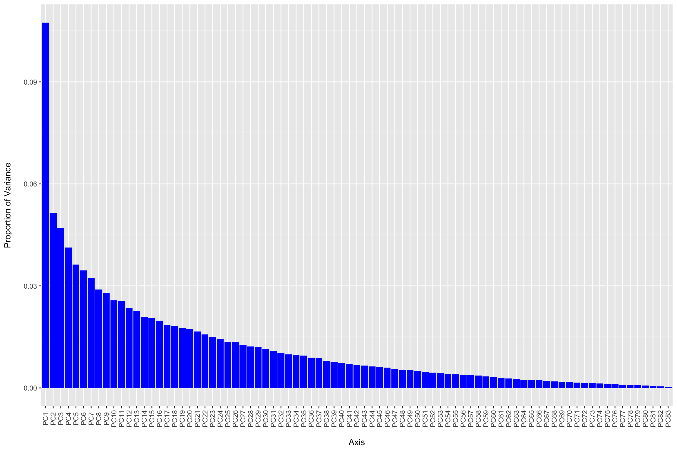
#Examine eigenvalues and % prop. variance explained
head(ord_clr$CA$eig)
## PC1 PC2 PC3 PC4 PC5 PC6
## 75.69204 36.27003 33.16649 29.08833 25.52986 24.32215sapply(ord_clr$CA$eig[1:5], function(x) x / sum(ord_clr$CA$eig)) ## PC1 PC2 PC3 PC4 PC5
## 0.10744095 0.05148344 0.04707812 0.04128939 0.03623832RDA without constraints is PCA…and we can generate the PCs using the phyloseq::ordinate function. A scree plot is then used to examine the proportion of total variation explained by each PC. Here we see that the first PC really stands out and then we have a gradual decline for the remaining components. You may hear people talk about looking for the “elbow” in the plot where the information plateaus to select the number of PCs to retain. Below we plot the first two components and scale the plot to reflect the relative amount of information explained by each axis as recommended by Nguyen and Holmes in their paper Ten quick tips for effective dimensionality reduction.
#Scale axes and plot ordination
clr1 <- ord_clr$CA$eig[1] / sum(ord_clr$CA$eig)
clr2 <- ord_clr$CA$eig[2] / sum(ord_clr$CA$eig)
phyloseq::plot_ordination(ps, ord_clr, type="samples", color="Status") +
  geom_point(size = 2) +
  coord_fixed(clr2 / clr1) +
  stat_ellipse(aes(group = Status), linetype = 2)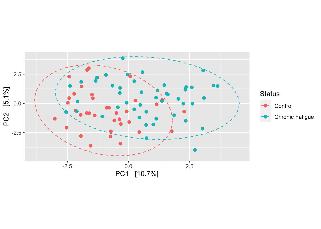
We see some separation between the chronic fatigue and healthy controls samples suggesting some differences in the communities according to sample type. There is also a fair degree of overlap as is often seen in clinical research studies examining the same environment in two different patient populations. While PCA is an exploratory data visualization tool, we can test whether the samples cluster beyond that expected by sampling variability using permutational multivariate analysis of variance (PERMANOVA). It does this by partitioning the sums of squares for the within- and between-cluster components using the concept of centroids. Many permutations of the data (i.e. random shuffling) are used to generate the null distribution. The test from ADONIS can be confounded by differences in dispersion (or spread)…so we want to check this as well.
#Generate distance matrix
clr_dist_matrix <- phyloseq::distance(ps_clr, method = "euclidean")
#ADONIS test
vegan::adonis(clr_dist_matrix ~ phyloseq::sample_data(ps_clr)$Status)
##
## Call:
## vegan::adonis(formula = clr_dist_matrix ~ phyloseq::sample_data(ps_clr)$Status)
##
## Permutation: free
## Number of permutations: 999
##
## Terms added sequentially (first to last)
##
## Df SumsOfSqs MeanSqs F.Model R2
## phyloseq::sample_data(ps_clr)$Status 1 2240 2240.17 3.2666 0.03831
## Residuals 82 56233 685.77 0.96169
## Total 83 58473 1.00000
## Pr(>F)
## phyloseq::sample_data(ps_clr)$Status 0.001 ***
## Residuals
## Total
## ---
## Signif. codes: 0 '***' 0.001 '**' 0.01 '*' 0.05 '.' 0.1 ' ' 1#Dispersion test and plot
dispr <- vegan::betadisper(clr_dist_matrix, phyloseq::sample_data(ps_clr)$Status)
dispr##
## Homogeneity of multivariate dispersions
##
## Call: vegan::betadisper(d = clr_dist_matrix, group =
## phyloseq::sample_data(ps_clr)$Status)
##
## No. of Positive Eigenvalues: 83
## No. of Negative Eigenvalues: 0
##
## Average distance to median:
## Control Chronic Fatigue
## 25.1 26.2
##
## Eigenvalues for PCoA axes:
## (Showing 8 of 83 eigenvalues)
## PCoA1 PCoA2 PCoA3 PCoA4 PCoA5 PCoA6 PCoA7 PCoA8
## 6282 3010 2753 2414 2119 2019 1895 1693plot(dispr, main = "Ordination Centroids and Dispersion Labeled: Aitchison Distance", sub = "")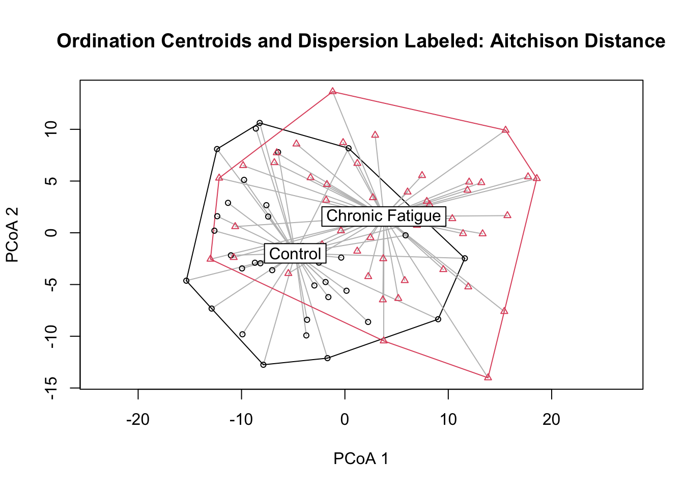
boxplot(dispr, main = "", xlab = "")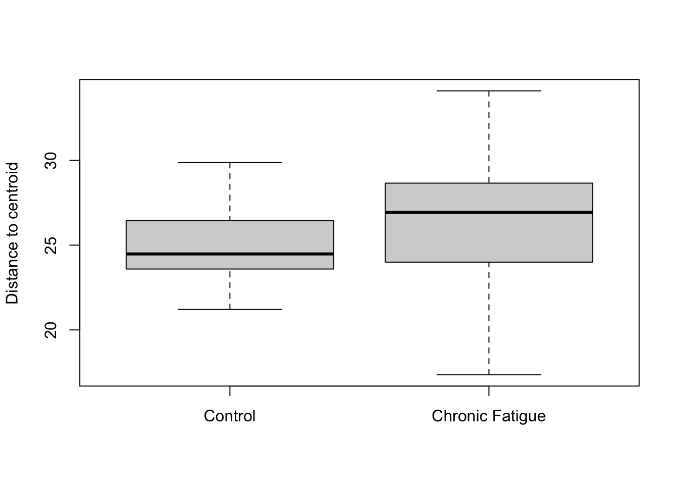
permutest(dispr)##
## Permutation test for homogeneity of multivariate dispersions
## Permutation: free
## Number of permutations: 999
##
## Response: Distances
## Df Sum Sq Mean Sq F N.Perm Pr(>F)
## Groups 1 24.95 24.9463 3.0491 999 0.075 .
## Residuals 82 670.89 8.1816
## ---
## Signif. codes: 0 '***' 0.001 '**' 0.01 '*' 0.05 '.' 0.1 ' ' 1We reject the null hypothesis of no difference in the centroid location according to Status. However, the proportion of variance explained is quite small. You might get slightly different numbers. This is because of the random process generating the permutations. There is a suggestion that the dispersion is greater in samples from patients with chronic fatigue syndrome. However, it does not exceed that expected by sampling variablilty at this sample size. As has been explained by others (Xia, Sun, and Chen; Ch 7.4), I want to mention that this type of testing is akin to attempting to “explain” the axes using metadata fields. A more formal approach to hypotheses testing can be done using redundancy analysis or canonical correspondence analysis that directly uses information on metadata fields when generating the ordinations and conducting testing. These approaches directly test hypotheses about environmental variables. I will not demonstrate these approaches here, but they can be computed using some of these same commands with minor modifications.
Lastly, I want to show you how you can bring in information the form of a phylogenic tree into beta-diversity analysis. The UniFrac metric incorporates phylogenic information by calculating the total branch lengths “unshared” between two samples divided by the total branch length. This approach often reveals interesting differences in the phylogenic relatedness between samples and sample types. Here we compute the weighted and unweighted UniFrac metrics using PCoA. PCoA can be thought of as PCA for non-Euclidian measures.
#Generate distances
ord_unifrac <- ordinate(ps_rare, method = "PCoA", distance = "wunifrac")
ord_unifrac_un <- ordinate(ps_rare, method = "PCoA", distance = "unifrac")
#Plot ordinations
a <- plot_ordination(ps_rare, ord_unifrac, color = "Status") + geom_point(size = 2)
b <- plot_ordination(ps_rare, ord_unifrac_un, color = "Status") + geom_point(size = 2)
cowplot::plot_grid(a, b, nrow = 1, ncol = 2, scale = .9, labels = c("Weighted", "Unweighted"))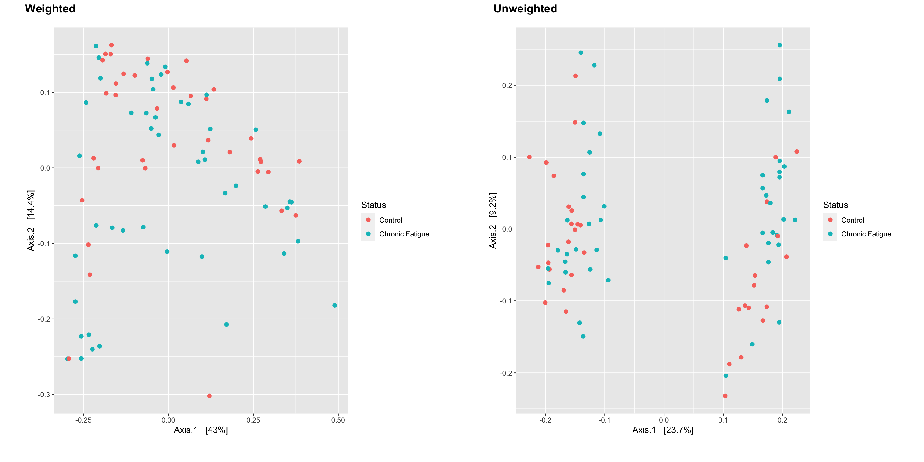
There is a large amount of overlap between sample types for the weighted UniFrac distance (accounts for the relative abundance of each of the taxa within the communities). However, there is clustering on at least the first axis for the unweighted UniFrac distance that is not “explained” by Status. Is there a metadata field in the data that reflects this separation? I’ll let you explore on your own.
Differential abundance testing
The goal of differential abundance testing is to identify specific taxa associated with clinical metadata variables of interest. This is a difficult task. It is also one of the more controversial areas in microbiome data analysis. Some of the reasons for this are described in a recent paper by James Morton et. al. in Nature Communications (2019), but is related to concerns that normalization and testing approaches have generally failed to control false discovery rates (here is a good example) and this has contributed to the lack of reproducibility in microbiome studies. If you think about it for a moment, a couple of difficulties come to mind:
- The goal of this type of analysis is to identify taxa that differ the most between conditions (or along a continuous gradient). Basically, we are identifying the most extreme results in the data. We would therefore expect some/many/most of these findings to have been “outlying” results simply due to chance sampling variation and to perhaps regress back towards the mean/null value when tested in a new sample of patients.
- The data are compositional and thus changes in one or more taxa can make it look like other/all taxa are changing. James Morton has an excellent example of this here. Methods that don’t properly account of the compositional nature of the data can have very high false discovery rates..
- Functionally redundant taxa may serve the same “niche” in different environments or populations causing different taxa to be identified as differentially abundant across samples (however the testing approach would not be what is misleading here).
- The high correlation between many taxa may cause different, but highly correlated, features to be selected in different studies.
Professor Frank Harrell provides a great overview of this general concern in Chapter 20 of his Biostatistics for Biomedical Research online text. For general thoughts on statistics and predictive modeling I highly recommend that you check out his blog and regression modeling strategies course notes.
Other fields have wrestled with similar problems and have introduced approaches such as the requirement of replicating results in multiple cohorts of patients prior to publication (or at least employing rigorous resampling approaches to gauge the reproducibility), analysis pre-specification, and focusing more on prediction than “naming names”. For compositional data including external information in the form of external spike-ins or estimates of total abundance (such as estimating total microbial load using qPCR), working with ratios, limiting the emphasis on testing, and understanding the limits of compositional data are likely reasonable ways forward here. However, none of these are a panacea. Methodologists working in the area of microbiome data analysis are addressing some of these issues, but there is still much work to be done. Two excellent recent papers you should check out include James Morton’s paper above and this preprint in biorxiv by McLaren, Willis and Callahan (2019) explaining and modeling correctable bias in metagenomic sequence studies.
In this section, I will present a two approaches for estimating differential abundance. The first is simply applying the non-parametric Wilcoxon rank-sum test to each taxon. The second is a version of the Wilcoxon test developed for compositional NGS data. I chose these two approaches since they are commonly used in microbiome studies and I expect many of you will have some familiarity with the Wilcoxon test or (Gosset’s) t-test. However, all results should be interpreted in light of the concerns raised above. I also include the use of a CoDA transform for both since there does seem to be some growing support that log-ratio methodologies may better control the false positive rate.
Many researchers will apply the non-parametric Wilcoxon rank-sum test to each OTU/ASV/species after normalization. We will do this here. We will also use nested data frames as advocated by Hadley Wickham to keep the data and test results together in a single data.frame. At first, I found this approach a little strange. However, I have come to use it all the time. It is perhaps a bit overkill here, but a very helpful framework when you want to run many models and then save them together with the data and results (especially when they take a long time to run). Here is a link to a complete description of the nested frame approach in the R for Data Science book. We also use the map function from purr. This operates like a for loop, allowing us to iterate the test over each OTU, but with less coding. This is a big chunk of code. I will talk you through it.
#Generate data.frame with OTUs and metadata
ps_wilcox <- data.frame(t(data.frame(phyloseq::otu_table(ps_clr))))
ps_wilcox$Status <- phyloseq::sample_data(ps_clr)$Status
#Define functions to pass to map
wilcox_model <- function(df){
  wilcox.test(abund ~ Status, data = df)
}
wilcox_pval <- function(df){
  wilcox.test(abund ~ Status, data = df)$p.value
}
#Create nested data frames by OTU and loop over each using map
wilcox_results <- ps_wilcox %>%
  gather(key = OTU, value = abund, -Status) %>%
  group_by(OTU) %>%
  nest() %>%
  mutate(wilcox_test = map(data, wilcox_model),
         p_value = map(data, wilcox_pval))
#Show results
head(wilcox_results)
## # A tibble: 6 x 4
## # Groups: OTU [6]
## OTU data wilcox_test p_value
## <chr> <list> <list> <list>
## 1 OTU1 <tibble [84 × 2]> <htest> <dbl [1]>
## 2 OTU2 <tibble [84 × 2]> <htest> <dbl [1]>
## 3 OTU3 <tibble [84 × 2]> <htest> <dbl [1]>
## 4 OTU4 <tibble [84 × 2]> <htest> <dbl [1]>
## 5 OTU5 <tibble [84 × 2]> <htest> <dbl [1]>
## 6 OTU6 <tibble [84 × 2]> <htest> <dbl [1]>head(wilcox_results$data[[1]])## # A tibble: 6 x 2
## Status abund
## <fct> <dbl>
## 1 Chronic Fatigue 1.29
## 2 Control 5.81
## 3 Control 5.62
## 4 Chronic Fatigue 6.23
## 5 Chronic Fatigue 9.47
## 6 Control 7.43wilcox_results$wilcox_test[[1]]##
## Wilcoxon rank sum exact test
##
## data: abund by Status
## W = 1172, p-value = 0.006066
## alternative hypothesis: true location shift is not equal to 0wilcox_results$p_value[[1]]## [1] 0.006066387Here we can see that we have a tibble where:
- each OTU is a row
- the data column contains a tibble for each OTU that contains the CLR abundance and Status fields (i.e. seperate data.frame for each OTU)
- the wilcox_test column contains the results of each Wilcoxon test
- the p_value column contains the extracted p-value for each test
Now we will unnest the results, grab the OTU names and p-values, add the taxonomic labels, and calculate the FDR adjusted p-values.
#Unnesting
wilcox_results <- wilcox_results %>%
  dplyr::select(OTU, p_value) %>%
  unnest()
## Warning: `cols` is now required when using unnest().
## Please use `cols = c(p_value)`head(wilcox_results)## # A tibble: 6 x 2
## # Groups: OTU [6]
## OTU p_value
## <chr> <dbl>
## 1 OTU1 0.00607
## 2 OTU2 0.0686
## 3 OTU3 0.830
## 4 OTU4 0.0130
## 5 OTU5 0.419
## 6 OTU6 0.258#Adding taxonomic labels
taxa_info <- data.frame(tax_table(ps_clr))
taxa_info <- taxa_info %>% rownames_to_column(var = "OTU")
#Computing FDR corrected p-values
wilcox_results <- wilcox_results %>%
full_join(taxa_info) %>%
arrange(p_value) %>%
mutate(BH_FDR = p.adjust(p_value, "BH")) %>%
filter(BH_FDR < 0.05) %>%
dplyr::select(OTU, p_value, BH_FDR, everything())## Joining, by = "OTU"#Printing results
print.data.frame(wilcox_results) ## OTU p_value BH_FDR Kingdom Phylum Class
## 1 OTU48 1.893126e-05 1.893126e-05 Bacteria Firmicutes Clostridia
## 2 OTU38 4.168412e-05 4.168412e-05 Bacteria Firmicutes Clostridia
## 3 OTU44 2.750125e-04 2.750125e-04 Bacteria Firmicutes Clostridia
## 4 OTU61 1.217944e-03 1.217944e-03 Bacteria Firmicutes Clostridia
## 5 OTU104 1.390580e-03 1.390580e-03 Bacteria Firmicutes Clostridia
## 6 OTU115 1.804359e-03 1.804359e-03 Bacteria Firmicutes Clostridia
## 7 OTU83 2.050647e-03 2.050647e-03 Bacteria Firmicutes Clostridia
## 8 OTU8 2.719699e-03 2.719699e-03 Bacteria Firmicutes Clostridia
## 9 OTU123 2.719699e-03 2.719699e-03 Bacteria Firmicutes Erysipelotrichi
## 10 OTU117 3.801488e-03 3.801488e-03 Bacteria Firmicutes Clostridia
## 11 OTU1 6.066387e-03 6.066387e-03 Bacteria Bacteroidetes Bacteroidia
## 12 OTU133 6.420958e-03 6.420958e-03 Bacteria Actinobacteria Coriobacteriia
## 13 OTU26 8.720398e-03 8.720398e-03 Bacteria Actinobacteria Actinobacteria
## 14 OTU116 9.462190e-03 9.462190e-03 Bacteria Firmicutes Clostridia
## 15 OTU43 9.721528e-03 9.721528e-03 Bacteria Firmicutes Clostridia
## 16 OTU51 9.721528e-03 9.721528e-03 Bacteria Firmicutes Clostridia
## 17 OTU4 1.301459e-02 1.301459e-02 Bacteria Firmicutes Clostridia
## 18 OTU21 1.519295e-02 1.519295e-02 Bacteria Firmicutes Clostridia
## 19 OTU42 1.639651e-02 1.639651e-02 Bacteria Firmicutes Erysipelotrichi
## 20 OTU39 1.953122e-02 1.953122e-02 Bacteria Cyanobacteria Chloroplast
## 21 OTU17 2.051686e-02 2.051686e-02 Bacteria Firmicutes Clostridia
## 22 OTU113 2.102556e-02 2.102556e-02 Bacteria Firmicutes Clostridia
## 23 OTU112 2.261734e-02 2.261734e-02 Bacteria Firmicutes Clostridia
## 24 OTU33 2.431157e-02 2.431157e-02 Bacteria Firmicutes Clostridia
## 25 OTU99 2.550051e-02 2.550051e-02 Bacteria Firmicutes Clostridia
## 26 OTU64 2.673882e-02 2.673882e-02 Bacteria Firmicutes Clostridia
## 27 OTU130 2.673882e-02 2.673882e-02 Bacteria Firmicutes Clostridia
## 28 OTU102 3.372788e-02 3.372788e-02 Bacteria Bacteroidetes Bacteroidia
## 29 OTU53 4.037823e-02 4.037823e-02 Bacteria Firmicutes Clostridia
## 30 OTU49 4.220272e-02 4.220272e-02 Bacteria Firmicutes Clostridia
## 31 OTU76 4.220272e-02 4.220272e-02 Bacteria Firmicutes Clostridia
## 32 OTU101 4.706752e-02 4.706752e-02 Bacteria Bacteroidetes Bacteroidia
## 33 OTU135 4.706752e-02 4.706752e-02 Bacteria Proteobacteria Alphaproteobacteria
## 34 OTU40 4.809443e-02 4.809443e-02 Bacteria Firmicutes Clostridia
## 35 OTU98 4.809443e-02 4.809443e-02 Bacteria Firmicutes Erysipelotrichi
## 36 OTU103 4.913987e-02 4.913987e-02 Bacteria Actinobacteria Coriobacteriia
## Order Family Genus
## 1 Clostridiales Lachnospiraceae Coprococcus
## 2 Clostridiales Ruminococcaceae Oscillospira
## 3 Clostridiales Lachnospiraceae [Ruminococcus]
## 4 Clostridiales Lachnospiraceae <NA>
## 5 Clostridiales Lachnospiraceae Blautia
## 6 Clostridiales [Mogibacteriaceae] <NA>
## 7 Clostridiales Lachnospiraceae Blautia
## 8 Clostridiales Lachnospiraceae [Ruminococcus]
## 9 Erysipelotrichales Erysipelotrichaceae Coprobacillus
## 10 Clostridiales Lachnospiraceae Dorea
## 11 Bacteroidales Porphyromonadaceae Parabacteroides
## 12 Coriobacteriales Coriobacteriaceae <NA>
## 13 Bifidobacteriales Bifidobacteriaceae Bifidobacterium
## 14 Clostridiales Ruminococcaceae <NA>
## 15 Clostridiales Lachnospiraceae <NA>
## 16 Clostridiales Lachnospiraceae <NA>
## 17 Clostridiales Lachnospiraceae [Ruminococcus]
## 18 Clostridiales Ruminococcaceae Ruminococcus
## 19 Erysipelotrichales Erysipelotrichaceae Clostridium
## 20 Streptophyta <NA> <NA>
## 21 Clostridiales Lachnospiraceae <NA>
## 22 Clostridiales Eubacteriaceae Anaerofustis
## 23 Clostridiales Lachnospiraceae Coprococcus
## 24 Clostridiales Lachnospiraceae Blautia
## 25 Clostridiales <NA> <NA>
## 26 Clostridiales Eubacteriaceae Pseudoramibacter_Eubacterium
## 27 Clostridiales Ruminococcaceae <NA>
## 28 Bacteroidales [Barnesiellaceae] <NA>
## 29 Clostridiales Ruminococcaceae Ruminococcus
## 30 Clostridiales [Mogibacteriaceae] <NA>
## 31 Clostridiales Lachnospiraceae Lachnospira
## 32 Bacteroidales Porphyromonadaceae Parabacteroides
## 33 RF32 <NA> <NA>
## 34 Clostridiales <NA> <NA>
## 35 Erysipelotrichales Erysipelotrichaceae [Eubacterium]
## 36 Coriobacteriales Coriobacteriaceae Collinsella
## Species
## 1 <NA>
## 2 <NA>
## 3 <NA>
## 4 <NA>
## 5 producta
## 6 <NA>
## 7 <NA>
## 8 <NA>
## 9 <NA>
## 10 <NA>
## 11 <NA>
## 12 <NA>
## 13 adolescentis
## 14 <NA>
## 15 <NA>
## 16 <NA>
## 17 torques
## 18 bromii
## 19 saccharogumia
## 20 <NA>
## 21 <NA>
## 22 <NA>
## 23 <NA>
## 24 <NA>
## 25 <NA>
## 26 <NA>
## 27 <NA>
## 28 <NA>
## 29 <NA>
## 30 <NA>
## 31 <NA>
## 32 distasonis
## 33 <NA>
## 34 <NA>
## 35 dolichum
## 36 stercorisHere we see that we have several Clostridiales organisms identified as differentially abundant. Next, we might use bootstrap resampling to see how often these results replicated in subsets of the data and calculate a measure of effect size. However, we will not do that here. Instead we will take a look at another approach that uses the Wilcoxon test on the CLR transformed data with some improvements in the treatment of zero values and presentation of effect size.
ANOVA-like differential expression (ALDEx2) is a popular CoDA method for differential abundance testing. ALDEx2 can be run via a single command; however, there are several steps that are occurring in the background. At a high-level, the steps include:
- Generate a large number (here n=128) of posterior probabilities for the observance of each taxon (i.e. output many data.frames where the counts have been converted to proportions). This is done by Monte-Carlo sampling from a Dirichlet distribution with a small non-zero prior to deal with zeros. The total read count therefore only contributes to the precision of the proportions.
- Apply the centered log-ratio transformation to each instance.
- Apply the Wilcoxon test to each taxon for each simulated instance.
- Estimate the effect size as the difference between conditions divided by the maximum difference within conditions averaging over all instances. Scaling the between group difference by the maximum within group difference gives us a standardized effect size measure.
- Obtain the expected p-values for each taxon by averaging over all instances.
- Apply the BH-FDR correction to control the false positive rate.
For a more through explanation see the ALDEx2 Bioconductor vignette.
Lets give it a try.
#Run ALDEx2
aldex2_da <- ALDEx2::aldex(data.frame(phyloseq::otu_table(ps)), phyloseq::sample_data(ps)$Status, test="t", effect = TRUE, denom="iqlr")
## aldex.clr: generating Monte-Carlo instances and clr values## operating in serial mode## computing iqlr centering## aldex.ttest: doing t-test## aldex.effect: calculating effect sizes#Plot effect sizes
ALDEx2::aldex.plot(aldex2_da, type="MW", test="wilcox", called.cex = 1, cutoff = 0.05)
The output highlights the various steps for the ALDEx2 workflow. The interquartile log-ratio (iqlr) centering uses as the basis for the CLR transform the set of features that have variance values that fall between the first and third quartiles for all features in all groups in the dataset. This provides results that are more robust to asymmetric features between groups.
The effect size plot shows the median log2 fold difference by the median log2 dispersion. This is a measure of the effect size by the variability. Differentially abundant taxon will be those where the difference most exceeds the dispersion. Points toward the top of the figure are more abundant in CF samples while those towards the bottom are more abundant in healthy controls. Taxa with BH-FDR corrected p-values are shown in red. However, the authors state that:
We prefer to use the effect size whenever possible rather than statistical significance since an effect size tells the scientist what they want to know—“what is reproducibly different between groups”; this is emphatically not something that P values deliver. Now we will print the output with the taxonomic classifications appended. WE use the FDR p-values here to facilitate the comparison with the results from Wilcoxon test ran outside of ALDEx2.
#Clean up presentation
sig_aldex2 <- aldex2_da %>%
  rownames_to_column(var = "OTU") %>%
  filter(wi.eBH < 0.05) %>%
  arrange(effect, wi.eBH) %>%
  dplyr::select(OTU, diff.btw, diff.win, effect, wi.ep, wi.eBH)
sig_aldex2 <- left_join(sig_aldex2, taxa_info)
## Joining, by = "OTU"sig_aldex2## OTU diff.btw diff.win effect wi.ep wi.eBH Kingdom
## 1 OTU8 -2.307035 5.522587 -0.3839105 0.0015096450 0.039837292 Bacteria
## 2 OTU48 3.639216 6.528139 0.5283635 0.0025403967 0.042007768 Bacteria
## 3 OTU44 3.541267 6.324375 0.5296702 0.0013725146 0.031600961 Bacteria
## 4 OTU38 3.277257 4.696329 0.6206553 0.0000348666 0.004124241 Bacteria
## Phylum Class Order Family Genus Species
## 1 Firmicutes Clostridia Clostridiales Lachnospiraceae [Ruminococcus] <NA>
## 2 Firmicutes Clostridia Clostridiales Lachnospiraceae Coprococcus <NA>
## 3 Firmicutes Clostridia Clostridiales Lachnospiraceae [Ruminococcus] <NA>
## 4 Firmicutes Clostridia Clostridiales Ruminococcaceae Oscillospira <NA>Here we see that again that several Clostridiales organisms are identified as differentially abundant. Consistent with the results of running the Wilcoxon test outside of ALDEx2, we see that OTU48, OTU38, OTU44, and OTU8 are listed as differentially abundant. The others do not reach the FDR cut-off used here; although, they likely have “largish” effect sizes. Try and see if you can obtain these values. The reason for the discrepancy is hard to discern, but may be related to differences in the use of the CLR basis (geometric mean of all taxa versus the IQLR) and/or the use of the Bayesian resampling with a non-zero prior.
Often, if I consider performing DA testing, I will run several models and focus on the intersection of OTUs and try to gain some insight into how the different normalization and/or models many be influencing the results.
There are MANY other approaches that can be used to attempt to identify differently abundant taxa. Some that are popular, or that I find interesting, and can be implemented in R include:
- Count Regression for Correlated Observations with the Beta-binomial (corncob)
- MicrobiomeDDA
- DESeq2
- Analysis of Composition of Microbiomes (ANCOM)
Outside of R, a recently developed approach using multinomial regression via tensorflow and differential ranking looks promising.
Prediction
As discussed by Dr. Haslam in the first lecture, the majority of clinical microbiome studies, conducted to date, have been correlative or focused on predicting outcomes using taxonomic abundances as the feature set. The predictive utility of the human microbiome in health and disease is of great interest and numerous studies have reported the ability to predict outcomes from metagenomic data. For example, here are links to three studies suggesting taxonomic profiles in fecal samples may predict the occurrence of colorectal cancer (1, 2, 3).
As with differential abundance testing, there are many models or statistical learning approaches that can be applied to metagenomic data for the purpose of predicting an outcome. For binary outcomes, generating predicted probabilities for the outcome of interest using generalized linear models (GLMs) is one approach. Machine learning approaches have also been used extensively in microbiome research; however, these approaches may likely require much larger datasets than they have typically been trained on if our goal is reproducible results (the same likely goes for most studies using GLMs, etc.).
One challenge we face when building a predictive model from metagenomic data is that we often have more features (taxon) than we have samples. For example, if we are working with microbial strains we might have more than 10,000 features to consider. One way to define high-dimensional data is when p > n, where: p = number of features and n = the number of samples. In these instances, one approach forward to reduce the dimensionality of the data. We did this earlier when we used PCA to extract the first two PCs that explained the largest fraction of variably in our data. Using a subset of the PCs as predictors in a GLM is known as principal components regression. We will give this approach a try below. Another is to include all the features as predictors, but to shrink their effects towards zero (or sometimes shrink them entirely out of the model). These approaches go by names such as ridge regression, LASSO, elastic nets, etc. Bayesian models with skeptical priors also can work well here. We will use a form of penalization on the principal components regression model below to highlight this approach and address potential overfitting even with just three PCs at this sample size (which is likely too small for robust prediction). A helpful guide to think about how many features or samples one might require to develop a predictive model is to consider how much overfitting you are willing to accept. Here are links to two excellent papers describing sample size determinations for continuous and binary outcomes in predictive modeling.
We will also examine a CoDA greedy stepwise selection model using balances that I think is a lot of fun…and very user-friendly.
For those interested in general resources for prediction modeling I recommend:
- Frank Harrell’s Regression Modeling Stratagies website and textbook
- Ewout Steyerberg’s Clinical Prediction Models textbook for a bit more introductory text
- Max Kuhn’s Applied Predictive Modeling textbook
- James, Witten, Hastie, and Tibshirani’s An Introduction to Statistical Learning
First we will create a data.frame that contains the Status and the first 3 PCs from the centered-log ratio transformed abundance table we generated before. We will then plot the unconditional association for each PC with the outcome of CF versus control.
#Generate data.frame
clr_pcs <- data.frame(
  "pc1" = ord_clr$CA$u[,1],
  "pc2" = ord_clr$CA$u[,2],
  "pc3" = ord_clr$CA$u[,3],
  "Status" = phyloseq::sample_data(ps_clr)$Status
)
clr_pcs$Status_num <- ifelse(clr_pcs$Status == "Control", 0, 1)
head(clr_pcs)
## pc1 pc2 pc3 Status Status_num
## ERR1331793 0.02850343 -0.07709724 0.0938970408 Chronic Fatigue 1
## ERR1331872 -0.08156129 0.14193568 0.1155088427 Control 0
## ERR1331819 -0.19356039 -0.08436341 -0.1048722096 Control 0
## ERR1331794 -0.04193714 0.09705602 0.0110912849 Chronic Fatigue 1
## ERR1331851 0.09994410 0.05534786 -0.0005008101 Chronic Fatigue 1
## ERR1331834 -0.15577774 0.02921040 -0.0204667015 Control 0#Specify a datadist object (for rms)
dd <- datadist(clr_pcs)
options(datadist = "dd")
#Plot the unconditional associations
a <- ggplot(clr_pcs, aes(x = pc1, y = Status_num)) +
Hmisc::histSpikeg(Status_num ~ pc1, lowess = TRUE, data = clr_pcs) +
labs(x = "\nPC1", y = "Pr(Chronic Fatigue)\n")
b <- ggplot(clr_pcs, aes(x = pc2, y = Status_num)) +
Hmisc::histSpikeg(Status_num ~ pc2, lowess = TRUE, data = clr_pcs) +
labs(x = "\nPC2", y = "Pr(Chronic Fatigue)\n")
c <- ggplot(clr_pcs, aes(x = pc3, y = Status_num)) +
Hmisc::histSpikeg(Status_num ~ pc3, lowess = TRUE, data = clr_pcs) +
labs(x = "\nPC3", y = "Pr(Chronic Fatigue)\n")
cowplot::plot_grid(a, b, c, nrow = 2, ncol = 2, scale = .9, labels = "AUTO")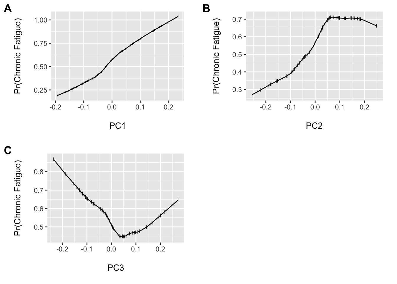
We see that we have the potential for some non-linear associations. Professor Harrell recommends that it is generally a good idea to assume some level of complexity since the penalty for allowing for a non-linear fit, when the association is in fact linear, is much less than when assuming linearity when the association is non-linear (i.e. you fit a straight line through a u-shaped curve). His rms package, along with the tidyverse, are the two packages I use most often and allows us to model this type of complexity easily using restricted cubic splines. These are a set of highly flexible, smoothly joined, piecewise polynomials entered for each variable. The number and placement of the knots helps control the flexibility. We will allow three knots for each term. However, this results in an additional 3 (6 total) model degrees of freedom…but we will shrink this down.
We first fit the full model and then perform a grid search to identify the optimum value for the penalty. We can also allow the penalty to differ for the simple and complex (i.e. nonlinear or interactions) terms. This is helpful if we want to allow for complexity, but down weight its impact. This would kind of be like adding more restrictive priors to the non-linear terms in a Bayesian model. We then plot the penalized log odds.
#Fit full model with splines (3 knots each)
m1 <- rms::lrm(Status_num ~ rcs(pc1, 3) + rcs(pc2, 3) + rcs(pc3, 3), data = clr_pcs, x = TRUE, y = TRUE)
#Grid search for penalties
pentrace(m1, list(simple = c(0, 1, 2), nonlinear = c(0, 100, 200)))
##
## Best penalty:
##
## simple nonlinear df
## 1 200 2.783027
##
## simple nonlinear df aic bic aic.c
## 0 0 6.000000 23.10845 8.523552 22.01754
## 0 100 3.049209 28.21043 20.798359 27.90157
## 1 100 2.810152 28.38363 21.552668 28.11659
## 2 100 2.641219 28.11811 21.697792 27.87875
## 0 200 3.024831 28.24577 20.892958 27.94131
## 1 200 2.783027 28.42060 21.655570 28.15810
## 2 200 2.611196 28.15166 21.804324 27.91706pen_m1 <- update(m1, penalty = list(simple = 1, nonlinear = 200))
pen_m1## Logistic Regression Model
##
## rms::lrm(formula = Status_num ~ rcs(pc1, 3) + rcs(pc2, 3) + rcs(pc3,
## 3), data = clr_pcs, x = TRUE, y = TRUE, penalty = list(simple = 1,
## nonlinear = 200))
##
##
## Penalty factors
##
## simple nonlinear interaction nonlinear.interaction
## 1 200 200 200
##
## Model Likelihood Discrimination Rank Discrim.
## Ratio Test Indexes Indexes
## Obs 84 LR chi2 33.99 R2 0.421 C 0.848
## 0 37 d.f. 2.783 g 1.759 Dxy 0.695
## 1 47 Pr(> chi2)<0.0001 gr 5.807 gamma 0.695
## max |deriv| 1e-12 Penalty 2.34 gp 0.322 tau-a 0.347
## Brier 0.159
##
## Coef S.E. Wald Z Pr(>|Z|) Penalty Scale
## Intercept 0.3458 0.2852 1.21 0.2254 0.0000
## pc1 11.6489 2.8714 4.06 <0.0001 0.1098
## pc1' 0.1202 0.9287 0.13 0.8970 1.0715
## pc2 6.4946 2.5132 2.58 0.0098 0.1098
## pc2' -0.0015 0.7643 0.00 0.9984 1.2987
## pc3 -3.8538 2.5659 -1.50 0.1331 0.1098
## pc3' 0.0259 1.0080 0.03 0.9795 0.9856
## #Plot log odds
ggplot(Predict(pen_m1))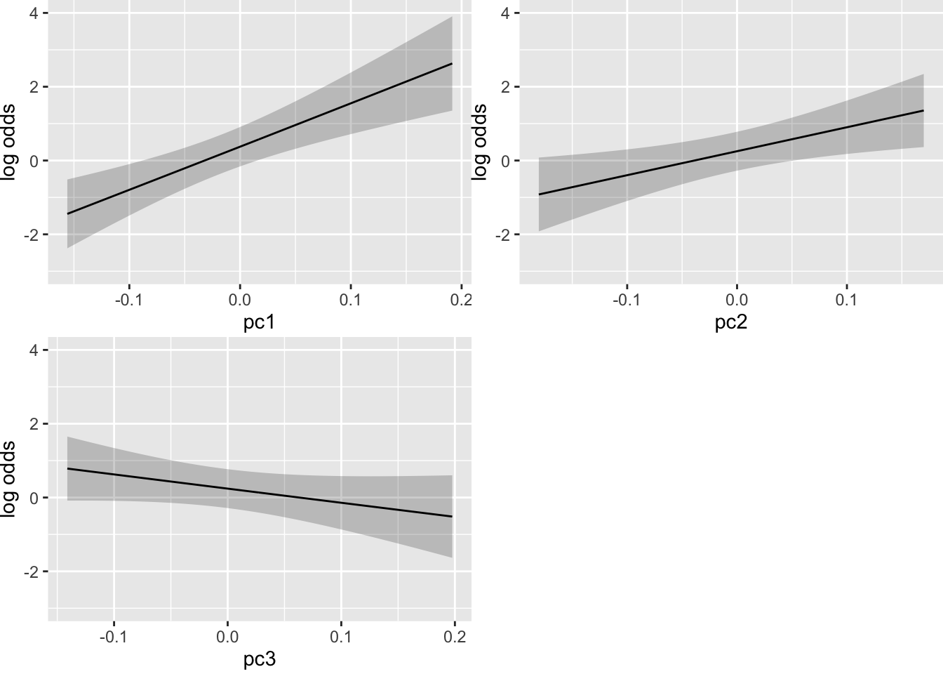
We can see from the value of the penalties and the resultant log odds that the conditional associations are quite linear. However, we will leave in the cubic spline terms to fully account for the degrees of freedom we entertained in the model building process. The optimal penalties were 1 for the simple and 200 for the non-linear terms (higher is better for the corrected AIC) and the effective degrees of freedom shrunk to 2.78. We won’t interpret the coefficients here since we purposefully biased them towards zero.
The Brier score is 0.16 and provides a measure of the mean squared difference between the predicted probabilities and actual outcomes. Thus, it is a quadratic proper scoring rule. The c-statistic is analogous to the area under the receiver operating characteristic curve and is a measure of rank discrimination. Here it is c = 0.85.
No we will perform bootstrap resampling to obtain an out-of-sample estimate of model performance. Here is a link describing this in greater detail.
#Obtain optimism corrected estimates
(val <- rms::validate(pen_m1))
## index.orig training test optimism index.corrected n
## Dxy 0.6952 0.7248 0.6817 0.0431 0.6521 40
## R2 0.4206 0.4536 0.4295 0.0240 0.3965 40
## Intercept 0.0000 0.0000 -0.0250 0.0250 -0.0250 40
## Slope 1.0000 1.0000 1.0265 -0.0265 1.0265 40
## Emax 0.0000 0.0000 0.0100 0.0100 0.0100 40
## D 0.3927 0.4045 0.3749 0.0297 0.3630 40
## U -0.0238 -0.0238 -0.0073 -0.0165 -0.0073 40
## Q 0.4165 0.4283 0.3822 0.0461 0.3704 40
## B 0.1589 0.1481 0.1647 -0.0166 0.1755 40
## g 1.7591 1.9083 1.9158 -0.0075 1.7666 40
## gp 0.3218 0.3287 0.3363 -0.0076 0.3293 40#Compute corrected c-statistic
(c_opt_corr <- 0.5 * (val[1, 5] + 1))## [1] 0.8260443#Plot calibration
cal <- rms::calibrate(pen_m1, B = 200)
plot(cal)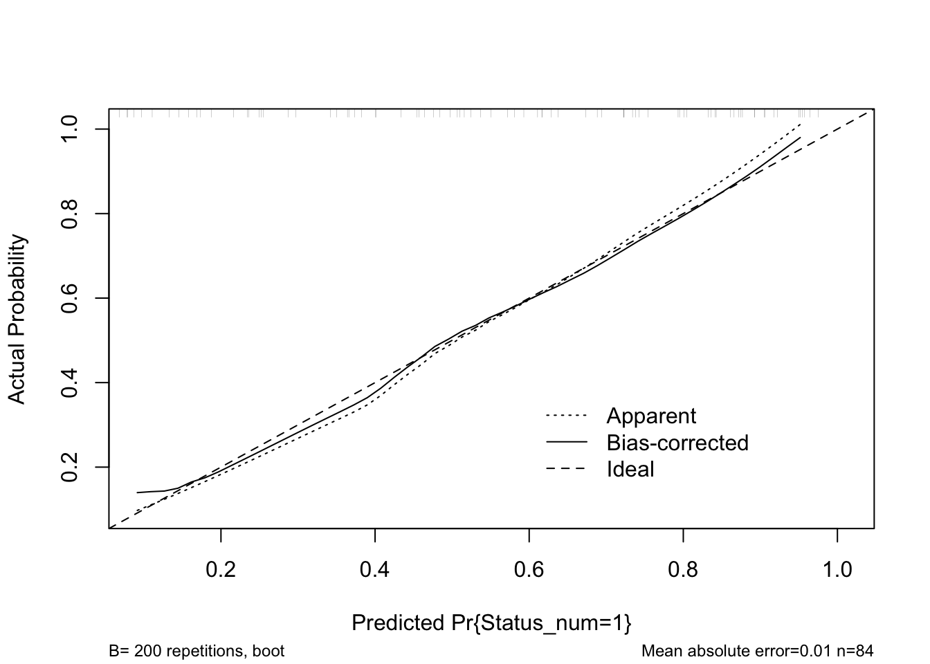
##
## n=84   Mean absolute error=0.01   Mean squared error=0.00018
## 0.9 Quantile of absolute error=0.024
#Output pred. probs
head(predict(pen_m1, type ="fitted"))## [1] 0.4560689 0.4689260 0.1137757 0.6098891 0.8683044 0.2314747We can see here that the Brier score is only mildly increased, and the c-statistic mildly decreased with repeated resampling. The calibration curve shows that the predictions are near the ideal across the range of predicted values. All-in-all this suggests we may expect to be able to predict patients with chronic fatigue from healthy controls with reasonable accuracy in a new sample of patients drawn from a similar population using just the three top PCs.
Now we will quickly show selbal as an alternaitve. From the documentation selbal is described as:
selbal is an R package for selection of balances in microbiome compositional data. As described in Rivera-Pinto et al. 2018 Balances: a new perspective for microbiome analysis https://doi.org/10.1101/219386, selbal implements a forward-selection method for the identification of two groups of taxa whose relative abundance, or balance, is associated with the response variable of interest. It requires much less typing…so let’s give it a go. This approach is computationally expensive (especially with larger datasets). So below we only use 1 repeat of 5-fold cross-validation to tune the selections. In practice, we would want to turn these numbers up to get better estimates. We will also aggregate the taxa to the family-level to speed up the computation.
#Agglomerate taxa
(ps_family <- phyloseq::tax_glom(ps, "Family"))
## phyloseq-class experiment-level object
## otu_table() OTU Table: [ 30 taxa and 84 samples ]
## sample_data() Sample Data: [ 84 samples by 23 sample variables ]
## tax_table() Taxonomy Table: [ 30 taxa by 7 taxonomic ranks ]
## phy_tree() Phylogenetic Tree: [ 30 tips and 29 internal nodes ]
## refseq() DNAStringSet: [ 30 reference sequences ]phyloseq::taxa_names(ps_family) <- phyloseq::tax_table(ps_family)[, "Family"]
#Run selbal
cv_sebal <- selbal::selbal.cv(x = data.frame(t(data.frame(phyloseq::otu_table(ps_family)))),
y = phyloseq::sample_data(ps_family)$Status,
n.fold = 5, n.iter = 1) ##
##
## ###############################################################
## STARTING selbal.cv FUNCTION
## ###############################################################
##
## #-------------------------------------------------------------#
## # ZERO REPLACEMENT . . .
##
##
## , . . . FINISHED.
## #-------------------------------------------------------------#
##
## #-------------------------------------------------------------#
## # Starting the cross - validation procedure . . .
## . . . finished.
## #-------------------------------------------------------------#
## ###############################################################
##
## The optimal number of variables is: 2
##
##
##
## ###############################################################
## . . . FINISHED.
## ################################################################plot/print results
cv_sebal$accuracy.nvar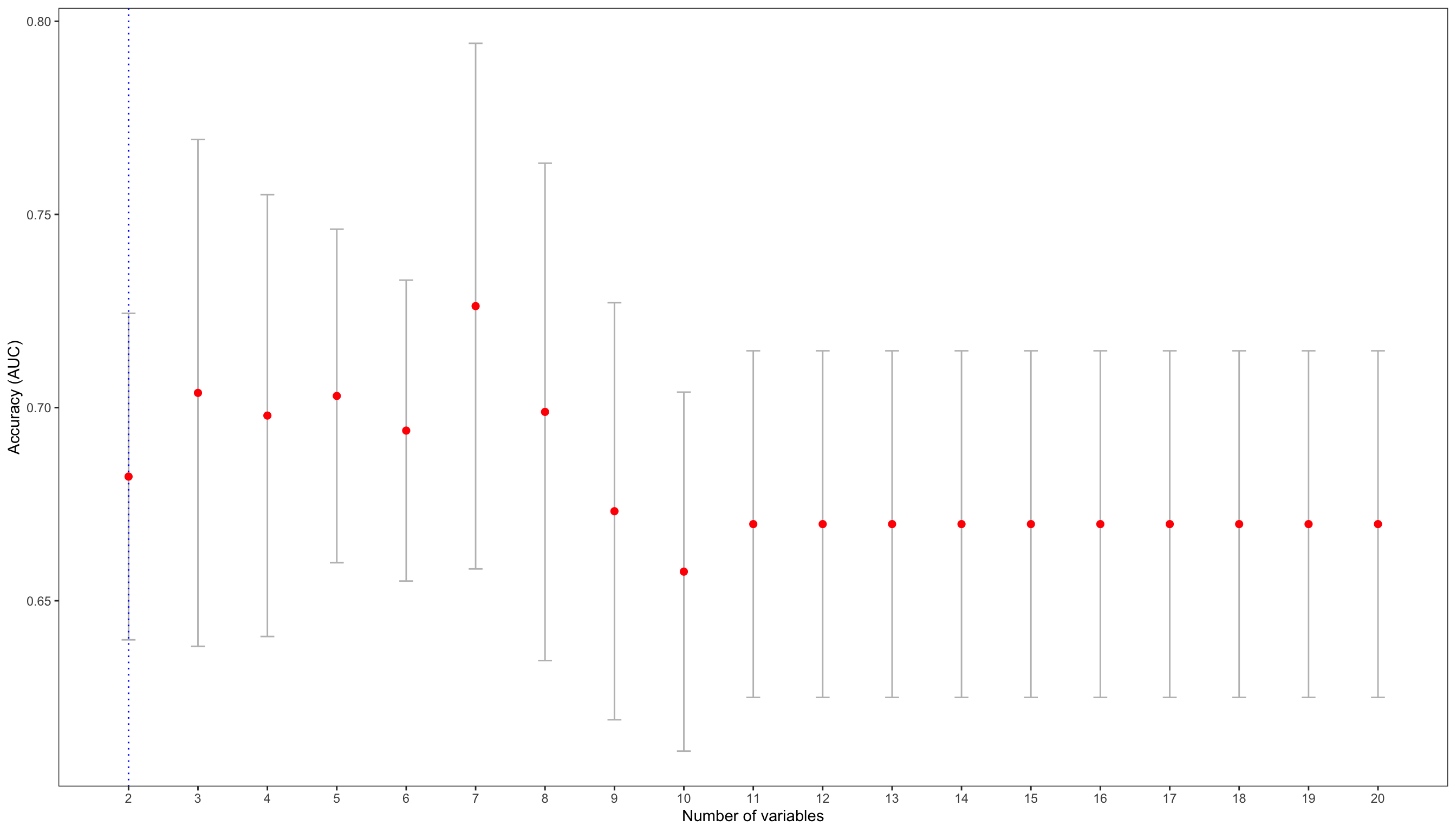
plot.new()
grid.draw(cv_sebal$global.plot)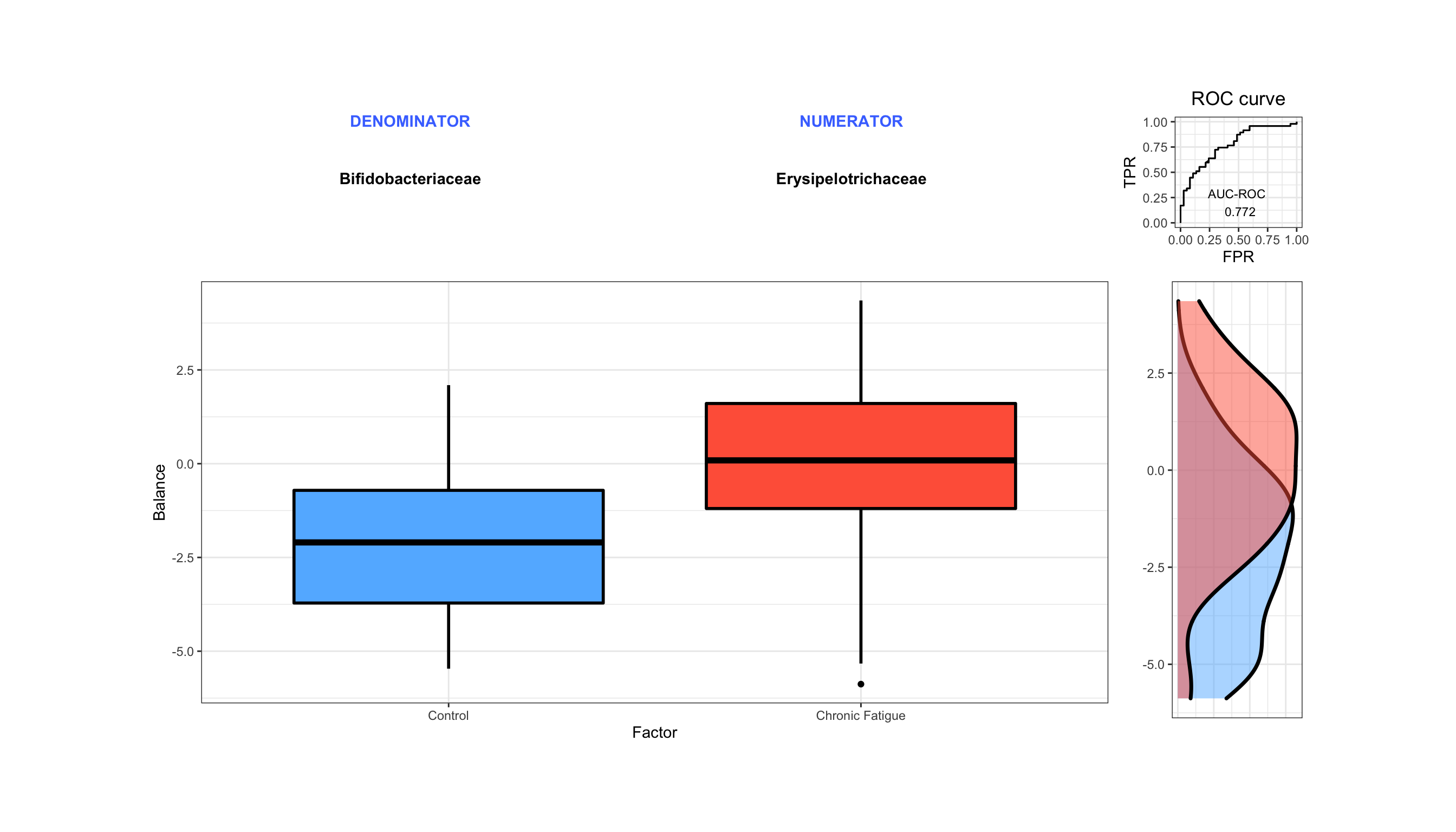
Here we can see that the cross-validation selected the two balance object as having “among” the best rank-discrimination. It selected the balance with erysipelotrichaceae in the numerator and bifidobacteriaceae in the denominator. So a higher relative abundance of erysipelotrichaceae to bifidobacteriaceae was among the most informative balances. The AUC was 0.77, but as low as AUC = 0.68 with 1 repeat of 5 fold cross-validation.
Give the model a try on the full ps object on your own. It should run in ~5 min on a standard laptop. How does the performance compare? Would you expect these results to be as reproducible as the GLM we fit? Why?