Bootstrap Resampling for Ranking Differentially Abundant Taxa
Microbiome studies often seek to identify individual features (i.e., OTUs/ASVs, species, pathways, etc.) associated some condition (i.e., exposure, experimental treatment, etc.) of interest. This problem can be approached in many different ways, but most commonly, one-at-a-time (OaaT) feature screening is undertaken. With OaaT screening, differences in species abundance according to some condition are obtained for each species individually, and the resultant associations ranked according to some measure. This measure is often the false discovery rate corrected p-value and the approach is referred to as differential abundance (DA) testing. In previous posts, I have highlighted some popular workflows to do this and touched on some of the difficulties.
While I often employ this type of approaches in my own work, I have limited confidence one can accurately identify the “correct set” of features from the typically long list of highly correlated and compositionally constrained features without some type of rigorous validation (which is not without its own difficulties as features may be expected to differ over time, geography, etc.). Rarely is such validation undertaken in the published literature, resulting in a possibly high proportion of findings that will not be reproduced in future studies.
Given access to validation samples is often difficult to come by if not pre-planned, and even if planned difficult to implement in practice due to resource and budgetary constraints, I have been thinking more about approaches that may help quantify the uncertainty in our ranking of the “most differently abundant features”. As usual, Professor Frank Harrell has some wisdom to share on this topic in Chapter 20 of his text Biostatistics for Biomedical Research titled Challenges of Analyzing High-Dimensional Data. He discusses several issues faced when attempting to perform feature selection with high-dimensional data including screening, multiplicity corrections, and ranking and recommendations bootstrap resampling as an approach to better reflect the difficulty of this task. He writes:
Feature discovery is really a ranking and selection problem. But ranking and selection methods are almost never used. An example bootstrap analysis on simulated data is presented later. This involves sampling with replacement from the combined (X, Y) dataset and recomputing for each bootstrap repetition the p association measures for the p candidate Xs. The p association measures are ranked. The ranking of each feature across bootstrap resamples is tracked, and a 0.95 confidence interval for the rank is derived by computing the 0.025 and 0.975 quantiles of the estimated ranks.
This approach puts OaaT in an honest context that fully admits the true difficulty of the task, including the high cost of the false negative rate (low power). Suppose that features are ranked so that a low ranking means weak estimated association and a high ranking means strong association. If one were to consider features to have “passed the screen” if their lower 0.95 confidence limit for their rank exceeds a threshold, and only dismisses features from further consideration if the upper confidence limit for their rank falls below a threshold, there would correctly be a large middle ground where features are not declared either winners or losers, and the researcher would be able to only make conclusions that are supported by the data.
This sounds like great advice. So in this post, I work through how one might implement this process in the hopes it might of use to others and future me. I found the results quite informative and look forward to applying the results to additional datasets. Below I:
- access publicly available data using the curatedMetagenomicData package
- convert the data into a phyloseq object for statistical analysis
- perform DA testing using the popular Maaslin2 package with default settings
- bootstrap the phyloseq object by sampling with replacement many times
- fit the Maaslin2 model to each bootstrap resample and obtaining a ranking for each feature
- present the 95% confidence interval for the ranks together with the Maaslin2 results
Load libraries
First, we load the required libraries.
library(curatedMetagenomicData); packageVersion("curatedMetagenomicData") ## [1] '3.0.10'library(tidyverse); packageVersion("tidyverse") ## [1] '1.3.1'library(phyloseq); packageVersion("phyloseq") ## [1] '1.36.0'library(Maaslin2); packageVersion("Maaslin2") ## [1] '1.6.0'library(future.apply); packageVersion("future.apply") ## [1] '1.8.1'library(Hmisc); packageVersion("Hmisc") ## [1] '4.6.0'Obtain example data
Then we pull down an example dataset using the curatedMetagenomicData package (this package is fantastic BTW and has been used in previous posts). This time we will select a study by Yachida et al. examining differences in the stool microbiomes of colorectal cancer patients and healthy controls via whole (meta)genome shotgun sequencing.
In the code chunks below, I identify the sample IDs of interest from the complete sampleMetadata object, use those IDs to pull down the processed taxonomic profiles as generated from MetaPhlAn 3, and then do a bit of data wrangling to convert the data into a phyloseq object for downstream analysis. I could have used the mia package for this last step, and likely will in future examples, to save some work and highlight some of its functionality (another awesome package).
meta_df <- curatedMetagenomicData::sampleMetadata

mydata <- meta_df %>%
  dplyr::filter(study_name == "YachidaS_2019") %>%
  dplyr::select(sample_id, subject_id, body_site, disease, age, gender, BMI) %>%
  dplyr::mutate(case_status = ifelse(disease == "CRC", "CRC",
                              ifelse(disease == "healthy", "Control", "Other"))) %>%
  dplyr::filter(case_status != "Other") %>%
  na.omit(.)

head(mydata)
## sample_id subject_id body_site disease age gender BMI case_status
## 1 SAMD00115014 sub_10021 stool CRC 57 male 26.88095 CRC
## 2 SAMD00115015 sub_10023 stool healthy 65 male 26.56250 Control
## 3 SAMD00115025 sub_10025 stool healthy 40 male 25.00000 Control
## 4 SAMD00115027 sub_10029 stool healthy 67 female 20.17325 Control
## 5 SAMD00114971 sub_10031 stool healthy 77 male 24.46460 Control
## 6 SAMD00114972 sub_10033 stool CRC 54 female 24.74745 CRCmydata %>%
dplyr::count(case_status)## case_status n
## 1 Control 245
## 2 CRC 258#building ps object
keep_id <- mydata$sample_id
crc_se_sp <- sampleMetadata %>%
dplyr::filter(sample_id %in% keep_id) %>%
curatedMetagenomicData::returnSamples("relative_abundance", counts = TRUE)
crc_sp_df <- as.data.frame(as.matrix(assay(crc_se_sp)))
crc_sp_df <- crc_sp_df %>%
rownames_to_column(var = "Species")
otu_tab <- crc_sp_df %>%
tidyr::separate(Species, into = c("Kingdom", "Phylum", "Class", "Order", "Family", "Genus", "Species"), sep = "\\|") %>%
dplyr::select(-Kingdom, -Phylum, -Class, -Order, -Family, -Genus) %>%
dplyr::mutate(Species = gsub("s__", "", Species)) %>%
tibble::column_to_rownames(var = "Species")
tax_tab <- crc_sp_df %>%
dplyr::select(Species) %>%
tidyr::separate(Species, into = c("Kingdom", "Phylum", "Class", "Order", "Family", "Genus", "Species"), sep = "\\|") %>%
dplyr::mutate(Kingdom = gsub("k__", "", Kingdom),
Phylum = gsub("p__", "", Phylum),
Class = gsub("c__", "", Class),
Order = gsub("o__", "", Order),
Family = gsub("f__", "", Family),
Genus = gsub("g__", "", Genus),
Species = gsub("s__", "", Species)) %>%
dplyr::mutate(spec_row = Species) %>%
tibble::column_to_rownames(var = "spec_row")
rownames(mydata) <- NULL
mydata <- mydata %>%
tibble::column_to_rownames(var = "sample_id")
(ps <- phyloseq(sample_data(mydata),
otu_table(otu_tab, taxa_are_rows = TRUE),
tax_table(as.matrix(tax_tab))))## phyloseq-class experiment-level object
## otu_table() OTU Table: [ 717 taxa and 503 samples ]
## sample_data() Sample Data: [ 503 samples by 7 sample variables ]
## tax_table() Taxonomy Table: [ 717 taxa by 7 taxonomic ranks ]head(sample_data(ps))## subject_id body_site disease age gender BMI case_status
## SAMD00115014 sub_10021 stool CRC 57 male 26.88095 CRC
## SAMD00115015 sub_10023 stool healthy 65 male 26.56250 Control
## SAMD00115025 sub_10025 stool healthy 40 male 25.00000 Control
## SAMD00115027 sub_10029 stool healthy 67 female 20.17325 Control
## SAMD00114971 sub_10031 stool healthy 77 male 24.46460 Control
## SAMD00114972 sub_10033 stool CRC 54 female 24.74745 CRCtable(sample_data(ps)$case_status)##
## Control CRC
## 245 258rm(list= ls()[!(ls() %in% c("ps"))])So you can see that we end up with a phyloseq object with 717 taxa from 503 samples of which n=258 samples are from participants with colorectal cancer and n=245 from otherwise healthy controls. We also have metadata on their age, sex, and BMI that we will include as model covariates (recognizing that this adjustment set is likely insufficient to fully account for confounding bias).
Performing DA testing with Maaslin2
Now that we have the data formatted for analysis, we can perform the DA testing using the popular Maaslin2 package with the default settings (as recommended here).
The second code chunk just cleans up the output a bit and recalculates the FDR p-value (q-value) given we are only interested in the results for case status.
m1 <- Maaslin2(
  input_data = data.frame(otu_table(ps)),
  input_metadata = data.frame(sample_data(ps)),
  output = "/Users/olljt2/desktop/maaslin2_output",
  min_abundance = 0.0,
  min_prevalence = 0.3,
  normalization = "TSS",
  transform = "LOG",
  analysis_method = "LM",
  fixed_effects = c("age", "gender", "BMI", "case_status"),
  correction = "BH",
  standardize = FALSE,
  cores = 1,
  plot_heatmap = FALSE,
  plot_scatter = FALSE
)
mas_res <- m1$results %>%
dplyr::filter(metadata == "case_status") %>%
dplyr::select(-qval, -name, -metadata, -N, -N.not.zero) %>%
dplyr::arrange(pval) %>%
dplyr::mutate(qval = p.adjust(pval, method = "fdr"))
head(mas_res)## feature value coef stderr pval
## 1 Collinsella_aerofaciens CRC 1.7494259 0.4378328 7.426711e-05
## 2 Roseburia_faecis CRC -1.7557381 0.4537057 1.234242e-04
## 3 Holdemania_filiformis CRC 1.1438006 0.3149170 3.102965e-04
## 4 Bacteroides_cellulosilyticus CRC 1.6620121 0.4732434 4.852776e-04
## 5 Streptococcus_anginosus_group CRC 0.8570658 0.2608184 1.087633e-03
## 6 Mogibacterium_diversum CRC 0.9275163 0.2956485 1.806511e-03
## qval
## 1 0.006603197
## 2 0.006603197
## 3 0.011067240
## 4 0.012981175
## 5 0.023275341
## 6 0.026898454
So based on these results, and assuming ranking these species on the FDR p-value is the goal, one might declare Collinsella aerofaciens the winner and celebrate victory! We also see several other species with low FDR p-values (go ahead and print the whole list to see the results for all taxa).
Most of the time we stop here and report the results. However, these results alone do not give us a good idea as to whether we might expect to achieve a similar ranking if we were to perform the same analysis in some new set of patient samples drawn from the “same source population”.
Bootstrap resampling can help give us some idea of the possible uncertainty in these rankings by treating the sample as if it were the population of interest and repeatedly sampling from it.
Bootstrap resampling and ranking
The first function below takes an existing phyloseq object as input, samples the data with replacement, and returns a single bootstrap resample as output. Combined with the replicate function, we can use this function to generate many bootstrap resamples (here n=500), and combine them all in a single list that we can then iterate over.
The second function fits the default Maaslin2 algorithm and ranks the results on the FDR p-values and effect sizes (i.e., coefficient values). We can then use the lapply function to apply the fucntion to the list of ps objects.
We then combine the results across the 500 resampled ps objects into a single data.frame so that we can operate on it to pull out the information of interest.
This will take a bit of time to run (~10 min on my laptop). I used the future package to allow the boostraping to operate in parallel. I did not for the model fitting.
ps_boot <- function(ps_object = ps){
  ps_ids <- sample_names(ps_object)
  boot_ids <- sample(ps_ids, size = length(ps_ids), replace = TRUE)
  boot_df <- data.frame(seq_id = boot_ids)


  meta_df <- data.frame(sample_data(ps_object)) %>%
    rownames_to_column(var = "seq_id")

  join_df <- left_join(boot_df, meta_df)


  otu_df <- data.frame(t(otu_table(ps_object))) %>%
    rownames_to_column(var = "seq_id")

  join_otu <- left_join(boot_df, otu_df)


  join_df <- join_df %>%
    mutate(boot_id = paste("S", row_number(), sep = "")) %>%
    dplyr::select(-seq_id) %>%
    column_to_rownames(var = "boot_id")

  join_otu <- join_otu %>%
    mutate(boot_id = paste("S", row_number(), sep = "")) %>%
    dplyr::select(-seq_id) %>%
    column_to_rownames(var = "boot_id") %>%
    t() %>%
    data.frame()

  boot_ps <- phyloseq(sample_data(join_df),
                      otu_table(join_otu, taxa_are_rows = TRUE))

  return(boot_ps)

}

get_ranks <- function(ps_object){
  m <- Maaslin2(
    input_data = data.frame(otu_table(ps_object)),
    input_metadata = data.frame(sample_data(ps_object)),
    output = "/Users/olljt2/desktop/maaslin2_output",
    min_abundance = 0.0,
    min_prevalence = 0.3,
    normalization = "TSS",
    transform = "LOG",
    analysis_method = "LM",
    fixed_effects = c("age", "gender", "BMI", "case_status"),
    correction = "BH",
    standardize = FALSE,
    cores = 1,
    plot_heatmap = FALSE,
    plot_scatter = FALSE)

  mas_out <- m$results %>%
    dplyr::filter(metadata == "case_status") %>%
    dplyr::select(-qval, -name, -metadata, -N, -N.not.zero) %>%
    dplyr::arrange(pval) %>%
    dplyr::mutate(qval = p.adjust(pval, method = "fdr"),
                  p_rank = rank(pval)) %>%
    dplyr::arrange(coef) %>%
    dplyr::mutate(coef_rank = rank(coef))

  return(mas_out)
}

availableCores()
plan(multisession)

boot_ps_list <- future_replicate(n = 500, expr = ps_boot(), simplify = FALSE, future.seed = 243)
boot_ranks <- lapply(boot_ps_list, get_ranks)
boot_ranks_df <- bind_rows(boot_ranks, .id = "column_label")
saveRDS(boot_ranks_df, "/users/olljt2/desktop/boot_ranks_df.rds")head(boot_ranks_df)## column_label feature value coef stderr pval
## 1 1 Lachnospira_pectinoschiza CRC -2.680995 0.5284147 5.518097e-07
## 2 1 Roseburia_faecis CRC -2.531921 0.4476999 2.623861e-08
## 3 1 Eubacterium_eligens CRC -2.320282 0.4878747 2.591016e-06
## 4 1 Bacteroides_dorei CRC -1.873865 0.5887274 1.549179e-03
## 5 1 Roseburia_intestinalis CRC -1.869300 0.4933628 1.698289e-04
## 6 1 Streptococcus_salivarius CRC -1.441700 0.3523627 4.998012e-05
## qval p_rank coef_rank
## 1 2.924592e-05 2 1
## 2 2.781293e-06 1 2
## 3 9.154924e-05 3 3
## 4 1.172950e-02 14 4
## 5 2.250233e-03 8 5
## 6 9.447558e-04 5 6So we can see that we now have a data.frame that contains the rankings of interest and an indicator for the resample from which the results were obtained.
Merge rank info
Here we compute the 95% CI for the ranks, as well as the highest and lowest rank for each species and merge it to the Maaslin2 results.
ranks_df <- boot_ranks_df %>%
  group_by(feature) %>%
  summarise(lcl_p_rank = round(quantile(p_rank, prob = (0.025)), 0),
            ucl_p_rank = round(quantile(p_rank, prob = (0.975)), 0),
            min_p_rank = min(p_rank),
            max_p_rank = max(p_rank),
            p_rank_95_ci = paste("(", lcl_p_rank, "; ", ucl_p_rank, ")", sep = "")) %>%
  dplyr::select(feature, p_rank_95_ci, min_p_rank, max_p_rank) %>%
  dplyr::ungroup()

mas_res_ranks <- dplyr::left_join(mas_res, ranks_df)
## Joining, by = "feature"Examine the rankings
head(mas_res_ranks)## feature value coef stderr pval
## 1 Collinsella_aerofaciens CRC 1.7494259 0.4378328 7.426711e-05
## 2 Roseburia_faecis CRC -1.7557381 0.4537057 1.234242e-04
## 3 Holdemania_filiformis CRC 1.1438006 0.3149170 3.102965e-04
## 4 Bacteroides_cellulosilyticus CRC 1.6620121 0.4732434 4.852776e-04
## 5 Streptococcus_anginosus_group CRC 0.8570658 0.2608184 1.087633e-03
## 6 Mogibacterium_diversum CRC 0.9275163 0.2956485 1.806511e-03
## qval p_rank_95_ci min_p_rank max_p_rank
## 1 0.006603197 (1; 34) 1 77
## 2 0.006603197 (1; 36) 1 69
## 3 0.011067240 (1; 42) 1 82
## 4 0.012981175 (1; 46) 1 70
## 5 0.023275341 (1; 53) 1 105
## 6 0.026898454 (1; 61) 1 96c_aerofaciens <- boot_ranks_df %>%
dplyr::filter(feature == "Collinsella_aerofaciens") %>%
dplyr::select(p_rank)
Hmisc::describe(c_aerofaciens)## c_aerofaciens
##
## 1 Variables 500 Observations
## --------------------------------------------------------------------------------
## p_rank
## n missing distinct Info Mean Gmd .05 .10
## 500 0 42 0.99 8.28 8.886 1.00 1.00
## .25 .50 .75 .90 .95
## 2.00 5.00 11.00 20.00 26.05
##
## lowest : 1 2 3 4 5, highest: 50 54 55 75 77
## --------------------------------------------------------------------------------We can see that there is quite a bit of variability in the 95% CI for the ranks of these top species including Collinsella aerofaciens.
From this, we might update our thinking as to whether this species may be expected to have the lowest FDR ranking if we tried this again in a new set of patient samples. It perhaps seems more plausible that it might be expected to fall somewhere around the top 30 or so. This is rather different, I think, than assuming that this is the “best hit” as based on these criteria and modeling approach etc. So depending where we set our thresholds for having “passed the screen”, we might have more or less enthusiasm for this species (or this DA testing approach in general). The ranks of these top species are quite similar (i.e., a lot of overlap), which is to be expected, since it is hard to pick true “winners”.
Go ahead and look at the distribution of rankings for all species. You will see that there is A LOT of overlap as you move further down the list highlighting the difficulty of the task we are trying to perform.
Let’s also plot the rankings for the top few species since I find this visualization often helpful. You may also want plot a few closer to the middle of the distribution just to see how disturbingly wide the variability can be (i.e., how the results could change from sample-to-sample).
ggplot(data = dplyr::filter(boot_ranks_df, feature == "Collinsella_aerofaciens"), aes(x = p_rank)) +
  geom_histogram(bins = 100, fill = "white", color = "dodgerblue") +
  labs(x = "\nRank", y = "Count\n")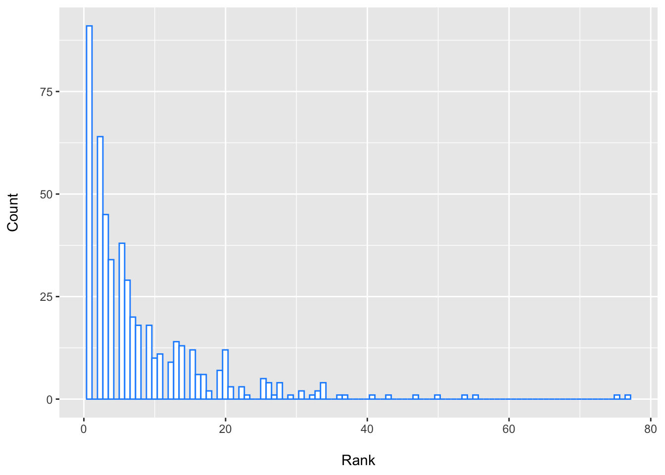
my_taxa <- c("Collinsella_aerofaciens", "Roseburia_faecis", "Holdemania_filiformis",
             "Bacteroides_cellulosilyticus", "Streptococcus_anginosus_group", "Mogibacterium_diversum")

ggplot(data = dplyr::filter(boot_ranks_df, feature %in% my_taxa), aes(x = p_rank, color = feature)) +
  geom_histogram(bins = 100) +
  labs(x = "\nRank", y = "Count\n") +
  facet_wrap(~feature) +
  theme(legend.position = "none")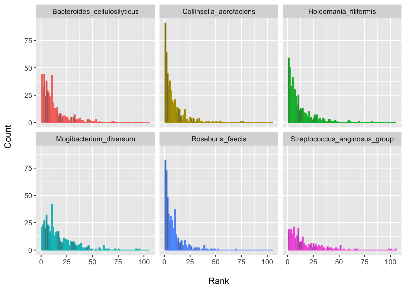
Other quantities from the bootstrap
We can also obtain many other quantities via bootstrapping. Here is just an example of how one might obtain the bootstrap SE (not that we need to here per se).
boot_ranks_df %>%
  dplyr::filter(feature %in% my_taxa) %>%
  dplyr::group_by(feature) %>%
  dplyr::summarise(boot_se = sd(coef)) %>%
  dplyr::arrange(feature)
## # A tibble: 6 × 2
## feature boot_se
## <chr> <dbl>
## 1 Bacteroides_cellulosilyticus 0.452
## 2 Collinsella_aerofaciens 0.453
## 3 Holdemania_filiformis 0.335
## 4 Mogibacterium_diversum 0.284
## 5 Roseburia_faecis 0.442
## 6 Streptococcus_anginosus_group 0.263head(mas_res) %>%
arrange(feature)## feature value coef stderr pval
## 1 Bacteroides_cellulosilyticus CRC 1.6620121 0.4732434 4.852776e-04
## 2 Collinsella_aerofaciens CRC 1.7494259 0.4378328 7.426711e-05
## 3 Holdemania_filiformis CRC 1.1438006 0.3149170 3.102965e-04
## 4 Mogibacterium_diversum CRC 0.9275163 0.2956485 1.806511e-03
## 5 Roseburia_faecis CRC -1.7557381 0.4537057 1.234242e-04
## 6 Streptococcus_anginosus_group CRC 0.8570658 0.2608184 1.087633e-03
## qval
## 1 0.012981175
## 2 0.006603197
## 3 0.011067240
## 4 0.026898454
## 5 0.006603197
## 6 0.023275341The main point of this post was just to share some thoughts on how bootstrapping and ranking may help us to think about the difficulty of feature selection in high-dimensions when trying to ascertain microbiome features that differ most according to some condition of interest. Bootstrap ranking is not a panacea, and the rankings will correlate with the FDR p-values, but considering the distribution of ranks might help us to think more about the limits of what we hope to learn from a single, often under-powered, study.
In the next post, I will show an example of how we can apply a meta-analysis approach to microbiome data when we do have access to several studies focused on the same condition. You may be surprised to see how the results from a single study can differ from those obtained from pooled estimates.
All the good ideas here on bootstrap ranking come from Frank. Any errors in logic or programming are my own.
Session Info
sessionInfo()## R version 4.1.1 (2021-08-10)
## Platform: x86_64-apple-darwin17.0 (64-bit)
## Running under: macOS Catalina 10.15.7
##
## Matrix products: default
## BLAS: /Library/Frameworks/R.framework/Versions/4.1/Resources/lib/libRblas.0.dylib
## LAPACK: /Library/Frameworks/R.framework/Versions/4.1/Resources/lib/libRlapack.dylib
##
## locale:
## [1] en_US.UTF-8/en_US.UTF-8/en_US.UTF-8/C/en_US.UTF-8/en_US.UTF-8
##
## attached base packages:
## [1] parallel stats4 stats graphics grDevices utils datasets
## [8] methods base
##
## other attached packages:
## [1] Hmisc_4.6-0 Formula_1.2-4
## [3] survival_3.2-11 lattice_0.20-44
## [5] future.apply_1.8.1 future_1.22.1
## [7] Maaslin2_1.6.0 phyloseq_1.36.0
## [9] forcats_0.5.1 stringr_1.4.0
## [11] dplyr_1.0.7 purrr_0.3.4
## [13] readr_2.0.2 tidyr_1.1.4
## [15] tibble_3.1.5 ggplot2_3.3.5
## [17] tidyverse_1.3.1 curatedMetagenomicData_3.0.10
## [19] TreeSummarizedExperiment_2.0.3 Biostrings_2.60.2
## [21] XVector_0.32.0 SingleCellExperiment_1.14.1
## [23] SummarizedExperiment_1.22.0 Biobase_2.52.0
## [25] GenomicRanges_1.44.0 GenomeInfoDb_1.28.4
## [27] IRanges_2.26.0 S4Vectors_0.30.2
## [29] BiocGenerics_0.38.0 MatrixGenerics_1.4.3
## [31] matrixStats_0.61.0
##
## loaded via a namespace (and not attached):
## [1] utf8_1.2.2 tidyselect_1.1.1
## [3] RSQLite_2.2.8 AnnotationDbi_1.54.1
## [5] htmlwidgets_1.5.4 grid_4.1.1
## [7] BiocParallel_1.26.2 munsell_0.5.0
## [9] codetools_0.2-18 withr_2.4.2
## [11] colorspace_2.0-2 filelock_1.0.2
## [13] highr_0.9 knitr_1.36
## [15] rstudioapi_0.13 robustbase_0.93-9
## [17] listenv_0.8.0 labeling_0.4.2
## [19] optparse_1.7.1 GenomeInfoDbData_1.2.6
## [21] lpsymphony_1.20.0 bit64_4.0.5
## [23] farver_2.1.0 rhdf5_2.36.0
## [25] parallelly_1.28.1 vctrs_0.3.8
## [27] treeio_1.16.2 generics_0.1.1
## [29] xfun_0.29 BiocFileCache_2.0.0
## [31] R6_2.5.1 bitops_1.0-7
## [33] rhdf5filters_1.4.0 cachem_1.0.6
## [35] DelayedArray_0.18.0 assertthat_0.2.1
## [37] promises_1.2.0.1 scales_1.1.1
## [39] nnet_7.3-16 gtable_0.3.0
## [41] globals_0.14.0 rlang_0.4.12
## [43] splines_4.1.1 lazyeval_0.2.2
## [45] broom_0.7.9 checkmate_2.0.0
## [47] BiocManager_1.30.16 yaml_2.2.1
## [49] reshape2_1.4.4 modelr_0.1.8
## [51] backports_1.2.1 httpuv_1.6.3
## [53] tools_4.1.1 bookdown_0.24
## [55] logging_0.10-108 ellipsis_0.3.2
## [57] jquerylib_0.1.4 biomformat_1.20.0
## [59] RColorBrewer_1.1-2 Rcpp_1.0.7
## [61] hash_2.2.6.1 plyr_1.8.6
## [63] base64enc_0.1-3 zlibbioc_1.38.0
## [65] RCurl_1.98-1.5 rpart_4.1-15
## [67] pbapply_1.5-0 haven_2.4.3
## [69] cluster_2.1.2 fs_1.5.0
## [71] magrittr_2.0.1 data.table_1.14.2
## [73] blogdown_1.7 reprex_2.0.1
## [75] mvtnorm_1.1-3 hms_1.1.1
## [77] mime_0.12 evaluate_0.14
## [79] xtable_1.8-4 jpeg_0.1-9
## [81] readxl_1.3.1 gridExtra_2.3
## [83] compiler_4.1.1 crayon_1.4.1
## [85] htmltools_0.5.2 mgcv_1.8-36
## [87] pcaPP_1.9-74 later_1.3.0
## [89] tzdb_0.1.2 lubridate_1.8.0
## [91] DBI_1.1.1 ExperimentHub_2.0.0
## [93] biglm_0.9-2.1 dbplyr_2.1.1
## [95] MASS_7.3-54 rappdirs_0.3.3
## [97] Matrix_1.3-4 ade4_1.7-18
## [99] getopt_1.20.3 permute_0.9-5
## [101] cli_3.1.0 igraph_1.2.7
## [103] pkgconfig_2.0.3 foreign_0.8-81
## [105] xml2_1.3.2 foreach_1.5.1
## [107] bslib_0.3.1 multtest_2.48.0
## [109] rvest_1.0.2 digest_0.6.28
## [111] vegan_2.5-7 rmarkdown_2.11
## [113] cellranger_1.1.0 tidytree_0.3.5
## [115] htmlTable_2.3.0 curl_4.3.2
## [117] shiny_1.7.1 lifecycle_1.0.1
## [119] nlme_3.1-152 jsonlite_1.7.2
## [121] Rhdf5lib_1.14.2 fansi_0.5.0
## [123] pillar_1.6.4 KEGGREST_1.32.0
## [125] fastmap_1.1.0 httr_1.4.2
## [127] DEoptimR_1.0-9 interactiveDisplayBase_1.30.0
## [129] glue_1.4.2 png_0.1-7
## [131] iterators_1.0.13 BiocVersion_3.13.1
## [133] bit_4.0.4 stringi_1.7.5
## [135] sass_0.4.0 blob_1.2.2
## [137] AnnotationHub_3.0.2 latticeExtra_0.6-29
## [139] memoise_2.0.0 ape_5.5