Applying Topic Models to Microbiome Data in R
Inherent limitations with one-at-a-time (OaaT) feature testing (i.e., single feature differential abundance analysis) have contributed to the increasing popularity of mixture models for correlating microbial features with factors of interest (i.e., phenotypes, environments, clinical measures, etc.). Latent Dirichlet allocation (LDA), popularized in the area of natural language processing (NLP) for topic modeling, seems to be among the most popular.
The application of LDA modeling to microbiome data is described in an excellent paper by Kris Sankaran and Susan Holmes, “Latent variable modeling for the microbiome”. A key advantage of LDA they highlight is that, opposed to Dirichlet multinomial mixture modeling, documents are allowed to have fractional membership across a set of topics. Thus, when applied to microbiome studies, samples are not exclusively classified to a given community type, but rather allowed to have fractional membership based on the probability of assignment.
To make the connection with text analyses clear (detailed description in the linked Sankaran and Holmes paper above) a:
- document = single microbiome sample
- term = single feature of the microbial samples. These are commonly taxa (i.e., species), genes, or ASVs/OTUs
- topic = community type (latent factor representing a community of features)
So at a high-level, the first goal of an LDA analysis applied to microbiome data is to derive topic-document probabilities and to convert them to observed read counts. Then one can apply existing tools developed for OaaT feature testing to identity differently abundant topics that (hopefully) capture associations for collections of microbes reflecting a given topic/community type.
The purpose of this post is not to get into the weeds of LDA (there are many good ones already out there), but rather to provide a high-level introduction as to to how one might implement such an approach. As new tools come online for this purpose, we expect to continue to update our workflows (for example utilizing alto for topic alignment, etc.). So check back with us for details.
In this example, we attempt to identify topics/community types associated with colorectal cancer (CRC) status using a popular, publicly available dataset contained in the curatedMetagenomicData package.
Loading libraries
First, we load the libraries we will require for the analysis.
library(curatedMetagenomicData); packageVersion("curatedMetagenomicData")## [1] '3.0.10'library(tidyverse); packageVersion("tidyverse") ## [1] '1.3.1'library(phyloseq); packageVersion("phyloseq") ## [1] '1.36.0'library(LinDA); packageVersion("LinDA") ## [1] '0.1.0'library(topicmodels); packageVersion("topicmodels") ## [1] '0.2.12'library(tidytext); packageVersion("tidytext") ## [1] '0.3.3'library(ldatuning); packageVersion("ldatuning") ## [1] '1.0.2'library(cowplot); packageVersion("cowplot") ## [1] '1.1.1'Downloading Yachida et. al. data
Then we grab an example data set. Here I use the YachidaS_2019 data provided in the curatedMetagenomicData package. For those of you who have read through some of my other posts, you can see that I use this dataset often. This is not for any particular reason other than it has a large number of samples and I now have some familiarity with it.
The code below pulls down the dataset and converts it into a phyloseq object for analysis. Then I filter out a few samples with lower sequencing depths and less common species.
meta_df <- curatedMetagenomicData::sampleMetadata

mydata <- meta_df %>%
  dplyr::filter(study_name == "YachidaS_2019") %>%
  dplyr::select(sample_id, subject_id, body_site, disease, age, gender, BMI) %>%
  dplyr::mutate(case_status = ifelse(disease == "CRC", "CRC",
                                     ifelse(disease == "healthy", "Control", "Other"))) %>%
  dplyr::filter(case_status != "Other") %>%
  na.omit(.)

keep_id <- mydata$sample_id

crc_se_sp <- sampleMetadata %>%
  dplyr::filter(sample_id %in% keep_id) %>%
  curatedMetagenomicData::returnSamples("relative_abundance", counts = TRUE)

crc_sp_df <- as.data.frame(as.matrix(assay(crc_se_sp)))

crc_sp_df <- crc_sp_df %>%
  rownames_to_column(var = "Species")

otu_tab <- crc_sp_df %>%
  tidyr::separate(Species, into = c("Kingdom", "Phylum", "Class", "Order", "Family", "Genus", "Species"), sep = "\\|") %>%
  dplyr::select(-Kingdom, -Phylum, -Class, -Order, -Family, -Genus) %>%
  dplyr::mutate(Species = gsub("s__", "", Species)) %>%
  tibble::column_to_rownames(var = "Species")

tax_tab <- crc_sp_df %>%
  dplyr::select(Species) %>%
  tidyr::separate(Species, into = c("Kingdom", "Phylum", "Class", "Order", "Family", "Genus", "Species"), sep = "\\|") %>%
  dplyr::mutate(Kingdom = gsub("k__", "", Kingdom),
                Phylum = gsub("p__", "", Phylum),
                Class = gsub("c__", "", Class),
                Order = gsub("o__", "", Order),
                Family = gsub("f__", "", Family),
                Genus = gsub("g__", "", Genus),
                Species = gsub("s__", "", Species)) %>%
  dplyr::mutate(spec_row = Species) %>%
  tibble::column_to_rownames(var = "spec_row")

rownames(mydata) <- NULL
mydata <- mydata %>%
  tibble::column_to_rownames(var = "sample_id")

(ps <- phyloseq(sample_data(mydata),
                otu_table(otu_tab, taxa_are_rows = TRUE),
                tax_table(as.matrix(tax_tab))))
## phyloseq-class experiment-level object
## otu_table() OTU Table: [ 717 taxa and 503 samples ]
## sample_data() Sample Data: [ 503 samples by 7 sample variables ]
## tax_table() Taxonomy Table: [ 717 taxa by 7 taxonomic ranks ]sample_data(ps)$read_count <- sample_sums(ps)
ps <- subset_samples(ps, read_count > 10^7)
minTotRelAbun <- 1e-5
x <- taxa_sums(ps)
keepTaxa <- (x / sum(x)) > minTotRelAbun
(ps <- prune_taxa(keepTaxa, ps))## phyloseq-class experiment-level object
## otu_table() OTU Table: [ 392 taxa and 500 samples ]
## sample_data() Sample Data: [ 500 samples by 8 sample variables ]
## tax_table() Taxonomy Table: [ 392 taxa by 7 taxonomic ranks ]head(sample_data(ps))## subject_id body_site disease age gender BMI case_status
## SAMD00115014 sub_10021 stool CRC 57 male 26.88095 CRC
## SAMD00115015 sub_10023 stool healthy 65 male 26.56250 Control
## SAMD00115025 sub_10025 stool healthy 40 male 25.00000 Control
## SAMD00115027 sub_10029 stool healthy 67 female 20.17325 Control
## SAMD00114971 sub_10031 stool healthy 77 male 24.46460 Control
## SAMD00114972 sub_10033 stool CRC 54 female 24.74745 CRC
## read_count
## SAMD00115014 51563815
## SAMD00115015 53302208
## SAMD00115025 44350874
## SAMD00115027 51661218
## SAMD00114971 41370786
## SAMD00114972 40155877table(sample_data(ps)$case_status)##
## Control CRC
## 243 257rm(list= ls()[!(ls() %in% c("ps"))])As you can see, we end up with a total of 392 species and 500 samples (n=243 controls and n=257 with CRC). This reflects a decent sized microbiome study by current standards.
Aggregating reads to genera
For this example, I reduce the number of taxa by agglomerating reads to genera to speed up the run time. However, this approach could be applied at any taxonomic level of interest (you just might spin out a larger number of topics when modeling species or genes).
(ps_g <- tax_glom(ps, taxrank = "Genus"))## phyloseq-class experiment-level object
## otu_table() OTU Table: [ 131 taxa and 500 samples ]
## sample_data() Sample Data: [ 500 samples by 8 sample variables ]
## tax_table() Taxonomy Table: [ 131 taxa by 7 taxonomic ranks ]taxa_names(ps_g) <- tax_table(ps_g)[, 6]
head(taxa_names(ps_g))## [1] "Faecalibacterium" "Eubacterium" "Parabacteroides" "Blautia"
## [5] "Agathobaculum" "Bifidobacterium"Selecting the number of topics
When fitting the LDA model we must specify the number of latent topics to model. There are various ways to go about this, but here we use the FindTopicsNumber function in the the ldatuning package (and two of the included metrics) to try to select an ideal number of features. More details can be found via the package and referenced papers. For these metrics a lower value suggests an optimal topic structure.
We also use the VEM method for speed. In practice, you may want to consider Gibbs sampling.
I modify the plotting function below to allow it to play well with cowplot.
count_matrix <- data.frame(t(data.frame(otu_table(ps_g))))

result <- FindTopicsNumber(
  count_matrix,
  topics = seq(from = 3, to = 50, by = 3),
  metrics = c("CaoJuan2009", "Arun2010"),
  method = "VEM",
  control = list(seed = 243),
  mc.cores = 4,
  verbose = TRUE
)
## fit models... done.
## calculate metrics:
## CaoJuan2009... done.
## Arun2010... done.my_plot <- function (values) #updating to allow plotting via cowplot::plot_grid
{
if ("LDA_model" %in% names(values)) {
values <- values[!names(values) %in% c("LDA_model")]
}
columns <- base::subset(values, select = 2:ncol(values))
values <- base::data.frame(values["topics"], base::apply(columns,
2, function(column) {
scales::rescale(column, to = c(0, 1), from = range(column))
}))
values <- reshape2::melt(values, id.vars = "topics", na.rm = TRUE)
values$group <- values$variable %in% c("Griffiths2004", "Deveaud2014")
values$group <- base::factor(values$group, levels = c(FALSE,
TRUE), labels = c("Minimize", "Maximize"))
p <- ggplot(values, aes_string(x = "topics", y = "value",
group = "variable"))
p <- p + geom_line()
p <- p + geom_point(aes_string(shape = "variable"), size = 3)
p <- p + guides(size = FALSE, shape = guide_legend(title = "Metrics:"))
p <- p + scale_x_continuous(breaks = values$topics)
p <- p + labs(x = "\nNumber of Topics", y = NULL)
p <- p + facet_grid(group ~ .)
p <- p + theme_bw() %+replace% theme(panel.grid.major.y = element_blank(),
panel.grid.minor.y = element_blank(), panel.grid.major.x = element_line(colour = "grey70"),
panel.grid.minor.x = element_blank(), legend.key = element_blank(),
strip.text.y = element_text(angle = 90),
legend.position = "bottom")
return(p)
}
(p1 <- my_plot(result))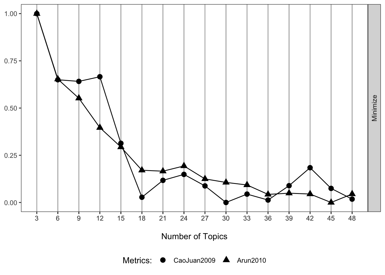
These metrics suggest that somewhere around 30 to 40 topics may be ideal. I go with 36 in this example.
Deriving topics via LDA
Now we use the LDA function in the topicmodels package to perform the LDA.
I use the tidytext package to extract the per-topic-per-word probabilities via the matrix = “beta” and the per-document-per-topic probabilities via the matrix = “gamma” arguments.
We can see that the per-document-per-topic probabilities shown below allow us to assign a probability for each topic to each sample. This is the fractional membership advantage described above.
lda_k36 <- LDA(count_matrix, k = 36, method = "VEM", control = list(seed = 243))

b_df <- data.frame(tidy(lda_k36, matrix = "beta"))

g_df <- data.frame(tidy(lda_k36, matrix = "gamma")) %>%
  arrange(document, topic)

head(b_df)
## topic term beta
## 1 1 Faecalibacterium 3.599927e-03
## 2 2 Faecalibacterium 4.468011e-04
## 3 3 Faecalibacterium 1.795527e-02
## 4 4 Faecalibacterium 2.448136e-05
## 5 5 Faecalibacterium 1.273613e-05
## 6 6 Faecalibacterium 1.403159e-05head(g_df)## document topic gamma
## 1 SAMD00114718 1 2.094965e-02
## 2 SAMD00114718 2 3.613434e-06
## 3 SAMD00114718 3 8.211247e-10
## 4 SAMD00114718 4 8.211251e-10
## 5 SAMD00114718 5 8.211255e-10
## 6 SAMD00114718 6 1.676575e-02Building the topic model phyloseq object
Now we just need to multiply the per-document-per-topic probabilities by the read count for each sample.
The code below does this and stores the data as a phyloseq object.
lib_size_df <- data.frame(sample_sums(ps_g)) %>%
  dplyr::rename("read_count" = "sample_sums.ps_g.") %>%
  rownames_to_column(var = "document")

tm_df <- left_join(lib_size_df, g_df) %>%
  mutate(topic_count = read_count * gamma,
         topic_count = round(topic_count, 0)) %>%
  dplyr::select(-read_count, -gamma) %>%
  pivot_wider(names_from = topic, values_from = topic_count) %>%
  dplyr::rename_with(~ paste0("Topic_", .), -document) %>%
  column_to_rownames(var = "document") %>%
  t(.) %>%
  data.frame(.)

(ps_topic_g <- phyloseq(
  sample_data(ps_g),
  otu_table(tm_df, taxa_are_rows = TRUE)))
## phyloseq-class experiment-level object
## otu_table() OTU Table: [ 36 taxa and 500 samples ]
## sample_data() Sample Data: [ 500 samples by 8 sample variables ]Fitting a DA model to the topics
Now that we have the data as read counts, we can use existing tools designed for differential abundance analysis to test for differentially abundant topics.
Here I use LinDA since it is fast, accommodates covariates, and has shown good performance when benchmarked against other methods.
FYI - I am using a slightly older version here that I load via the LinDA package. The function can now be found in the MicrobiomStat package. I include some prevalence filtering, trimming of extreme values, and covariate adjustment to highlight these options.
linda <- linda(otu.tab = data.frame(otu_table(ps_topic_g)), meta = data.frame(sample_data(ps_topic_g)),
               formula = '~ case_status + age + gender + BMI', alpha = 0.05, winsor.quan = 0.97,
               prev.cut = 0.3, lib.cut = 0, n.cores = 1)
## Pseudo-count approach is used.linda_res_df <- data.frame(linda$output$case_statusCRC) %>%
dplyr::arrange(padj) %>%
rownames_to_column(var = "Topic")
fdr_linda <- linda_res_df %>%
mutate(reject = ifelse(padj < 0.05, "Yes", "No")) %>%
separate(Topic, into = c("t", "t_n"), remove = FALSE, convert = TRUE) %>%
mutate(Topic = gsub("_", " ", Topic)) %>%
arrange(desc(t_n)) %>%
mutate(Topic = factor(Topic, levels = Topic))
(p2 <- ggplot(data = fdr_linda, aes(x = Topic, y = log2FoldChange, fill = reject)) +
geom_col(alpha = .8) +
labs(y = "\nLog2 Fold-Change", x = "") +
theme(axis.text.x = element_text(color = "black", size = 8),
axis.text.y = element_text(color = "black", size = 8),
axis.title.y = element_text(size = 8),
axis.title.x = element_text(size = 10),
legend.text = element_text(size = 8),
legend.title = element_text(size = 8)) +
coord_flip() +
scale_fill_manual(values = c("grey", "dodgerblue")) +
geom_hline(yintercept = 0, linetype="dotted") +
theme(legend.position = "none"))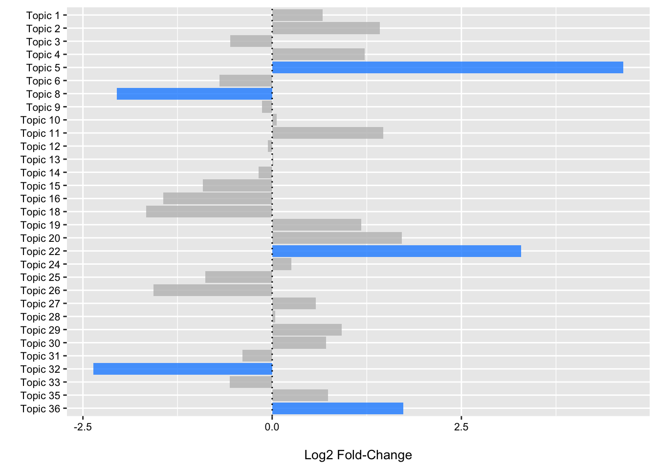
From the plot we can see that we have three topics that have positive log2 fold changes and low FDR p-values (< 0.05) for samples obtained from CRC patients when compared to controls. We have two that have negative log2 fold values and low FDR p-values highlighting enrichment of these topics in control samples.
In the next two sections, we will follow-up a bit on topic five.
Plotting per-topic-word-probabilities
Selecting topic five as an example, we can use the information in the per-topic-per-word probabilities matrix to examine which genera have the highest probabilities of assignment to this topic/community type.
Below we can see that Porphyromonas has the highest probability of assignment followed by several others with lower values.
b_plot <- b_df %>%
  dplyr::filter(topic == 5) %>%
  arrange(desc(beta)) %>%
  slice_head(n = 20) %>%
  arrange(desc(term)) %>%
  mutate(term = factor(term, levels = term))

(p3 <- ggplot(data = b_plot, aes(x = beta, y = term, color = term)) +
    geom_point(aes(size = beta)) +
    labs(x = "\nTopic 5: Genus-Topic Probabilities (beta)", y = "") +
    theme(legend.position = "none"))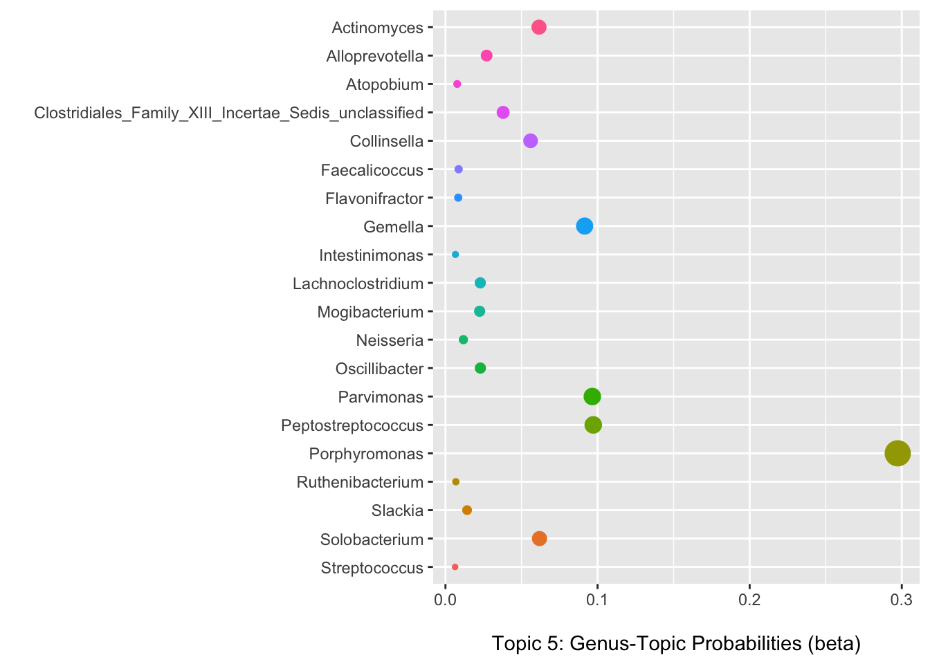
Plotting associations for the top contributing genera
We can also fit the LinDA model to each genera individually to get some idea of their association with CRC status when we do not directly account for the other features (for better or worse).
Here we see that nearly all of these genera are enriched in CRC samples (these plots could benefit from some focus on the variation as well). Thus, it makes sense that the community type would also have a strong, positive association as well.
linda_g_all <- linda(otu.tab = data.frame(otu_table(ps_g)), meta = data.frame(sample_data(ps_g)),
                      formula = '~ case_status + age + gender + BMI', alpha = 0.05, winsor.quan = 0.97,
                      prev.cut = 0, lib.cut = 0, n.cores = 1)
## Imputation approach is used.linda_res_g_df <- data.frame(linda_g_all$output$case_statusCRC) %>%
dplyr::arrange(padj) %>%
rownames_to_column(var = "Genus")
keep_g <- b_plot$term
log2_df <- linda_res_g_df %>%
filter(Genus %in% keep_g) %>%
arrange(desc(Genus)) %>%
mutate(Genus = factor(Genus, levels = Genus))
(p4 <- ggplot(data = log2_df, aes(x = Genus, y = log2FoldChange, fill = Genus)) +
geom_col(alpha = .8) +
labs(y = "\nLog2 Fold-Change", x = "") +
theme(axis.text.x = element_text(color = "black", size = 8),
axis.text.y = element_text(color = "black", size = 8),
axis.title.y = element_text(size = 8),
axis.title.x = element_text(size = 10),
legend.text = element_text(size = 8),
legend.title = element_text(size = 8)) +
coord_flip() +
geom_hline(yintercept = 0, linetype="dotted") +
theme(legend.position = "none"))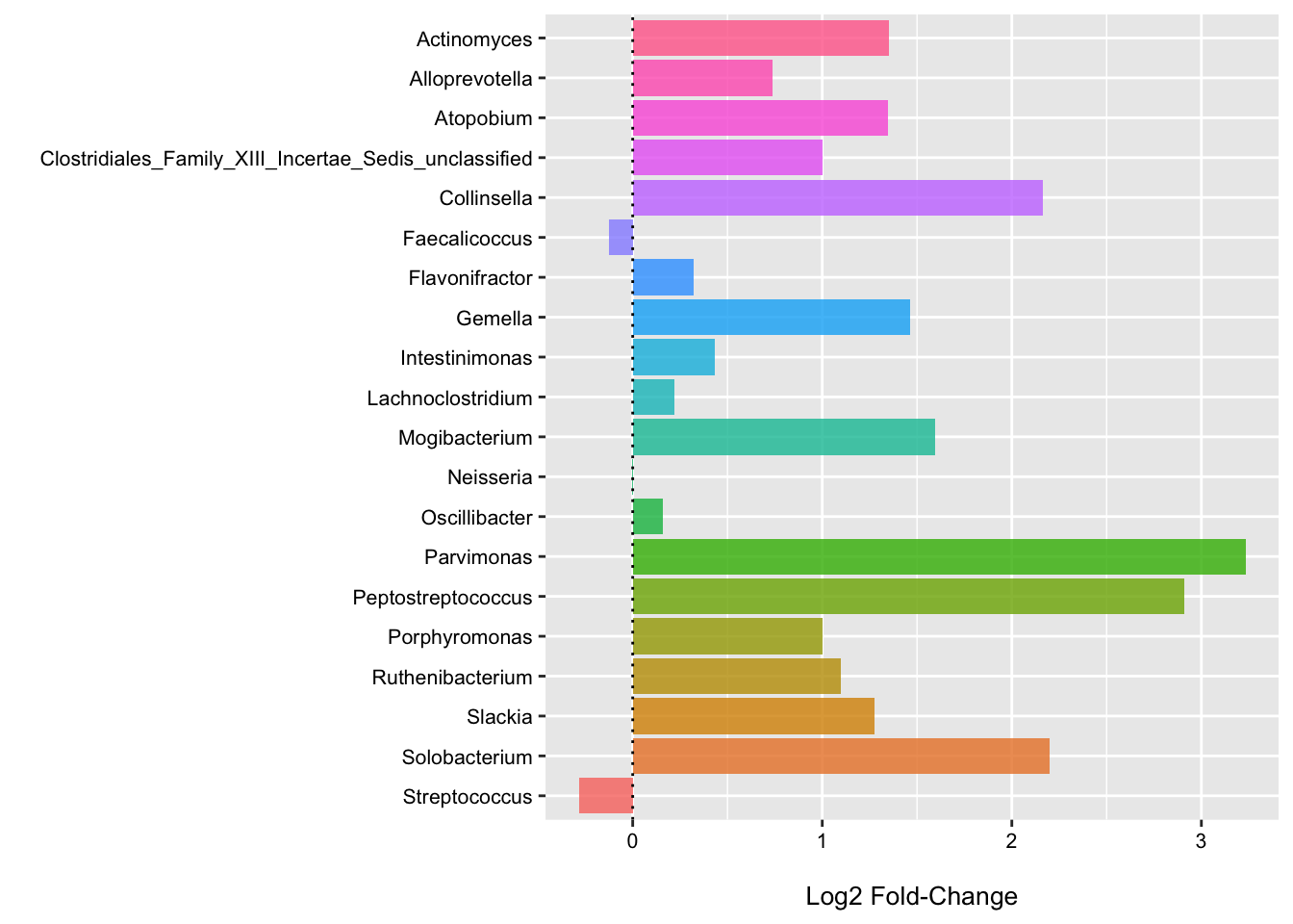
Example combined LDA figure
In this block I include some code to show how you might put all of this together in one figure.
cowplot::plot_grid(p1, p2, p3, p4, ncol = 2, nrow = 2, scale = .9, labels = c("A", "B", "C", "D")) +
  theme(plot.background = element_rect(fill = "white"))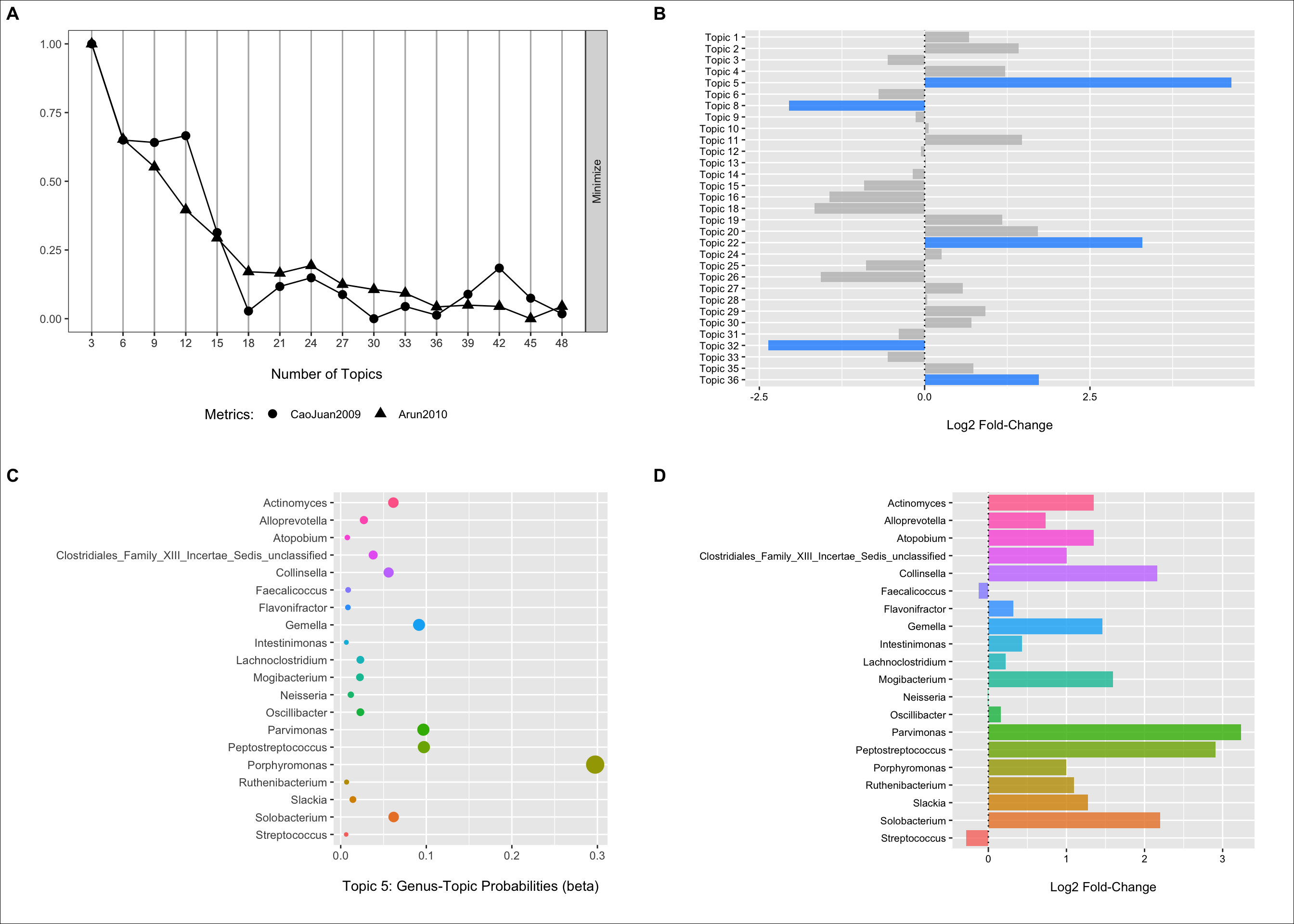
Session Info
sessionInfo()## R version 4.1.1 (2021-08-10)
## Platform: x86_64-apple-darwin17.0 (64-bit)
## Running under: macOS Catalina 10.15.7
##
## Matrix products: default
## BLAS: /Library/Frameworks/R.framework/Versions/4.1/Resources/lib/libRblas.0.dylib
## LAPACK: /Library/Frameworks/R.framework/Versions/4.1/Resources/lib/libRlapack.dylib
##
## locale:
## [1] en_US.UTF-8/en_US.UTF-8/en_US.UTF-8/C/en_US.UTF-8/en_US.UTF-8
##
## attached base packages:
## [1] parallel stats4 stats graphics grDevices utils datasets
## [8] methods base
##
## other attached packages:
## [1] cowplot_1.1.1 ldatuning_1.0.2
## [3] tidytext_0.3.3 topicmodels_0.2-12
## [5] LinDA_0.1.0 phyloseq_1.36.0
## [7] forcats_0.5.1 stringr_1.4.0
## [9] dplyr_1.0.7 purrr_0.3.4
## [11] readr_2.0.2 tidyr_1.1.4
## [13] tibble_3.1.5 ggplot2_3.3.5
## [15] tidyverse_1.3.1 curatedMetagenomicData_3.0.10
## [17] TreeSummarizedExperiment_2.0.3 Biostrings_2.60.2
## [19] XVector_0.32.0 SingleCellExperiment_1.14.1
## [21] SummarizedExperiment_1.22.0 Biobase_2.52.0
## [23] GenomicRanges_1.44.0 GenomeInfoDb_1.28.4
## [25] IRanges_2.26.0 S4Vectors_0.30.2
## [27] BiocGenerics_0.38.0 MatrixGenerics_1.4.3
## [29] matrixStats_0.61.0
##
## loaded via a namespace (and not attached):
## [1] utf8_1.2.2 tidyselect_1.1.1
## [3] lme4_1.1-27.1 RSQLite_2.2.8
## [5] AnnotationDbi_1.54.1 grid_4.1.1
## [7] BiocParallel_1.26.2 modeest_2.4.0
## [9] munsell_0.5.0 codetools_0.2-18
## [11] withr_2.4.2 colorspace_2.0-2
## [13] filelock_1.0.2 NLP_0.2-1
## [15] highr_0.9 knitr_1.36
## [17] rstudioapi_0.13 labeling_0.4.2
## [19] slam_0.1-48 GenomeInfoDbData_1.2.6
## [21] bit64_4.0.5 farver_2.1.0
## [23] rhdf5_2.36.0 fBasics_3042.89.1
## [25] vctrs_0.3.8 treeio_1.16.2
## [27] generics_0.1.1 xfun_0.29
## [29] BiocFileCache_2.0.0 R6_2.5.1
## [31] clue_0.3-60 bitops_1.0-7
## [33] rhdf5filters_1.4.0 cachem_1.0.6
## [35] DelayedArray_0.18.0 assertthat_0.2.1
## [37] promises_1.2.0.1 scales_1.1.1
## [39] gtable_0.3.0 spatial_7.3-14
## [41] timeDate_3043.102 rlang_0.4.12
## [43] splines_4.1.1 lazyeval_0.2.2
## [45] broom_0.7.9 BiocManager_1.30.16
## [47] yaml_2.2.1 reshape2_1.4.4
## [49] modelr_0.1.8 backports_1.2.1
## [51] httpuv_1.6.3 tokenizers_0.2.1
## [53] tools_4.1.1 bookdown_0.24
## [55] ellipsis_0.3.2 jquerylib_0.1.4
## [57] biomformat_1.20.0 stabledist_0.7-1
## [59] Rcpp_1.0.7 plyr_1.8.6
## [61] zlibbioc_1.38.0 RCurl_1.98-1.5
## [63] rpart_4.1-15 statip_0.2.3
## [65] haven_2.4.3 ggrepel_0.9.1
## [67] cluster_2.1.2 fs_1.5.0
## [69] magrittr_2.0.1 data.table_1.14.2
## [71] timeSeries_3062.100 blogdown_1.7
## [73] lmerTest_3.1-3 reprex_2.0.1
## [75] SnowballC_0.7.0 hms_1.1.1
## [77] mime_0.12 evaluate_0.14
## [79] xtable_1.8-4 readxl_1.3.1
## [81] compiler_4.1.1 crayon_1.4.1
## [83] minqa_1.2.4 htmltools_0.5.2
## [85] mgcv_1.8-36 later_1.3.0
## [87] tzdb_0.1.2 lubridate_1.8.0
## [89] DBI_1.1.1 ExperimentHub_2.0.0
## [91] rmutil_1.1.5 dbplyr_2.1.1
## [93] MASS_7.3-54 rappdirs_0.3.3
## [95] boot_1.3-28 Matrix_1.3-4
## [97] ade4_1.7-18 permute_0.9-5
## [99] cli_3.1.0 igraph_1.2.7
## [101] pkgconfig_2.0.3 numDeriv_2016.8-1.1
## [103] xml2_1.3.2 foreach_1.5.1
## [105] bslib_0.3.1 multtest_2.48.0
## [107] rvest_1.0.2 janeaustenr_0.1.5
## [109] digest_0.6.28 vegan_2.5-7
## [111] tm_0.7-8 rmarkdown_2.11
## [113] cellranger_1.1.0 tidytree_0.3.5
## [115] curl_4.3.2 shiny_1.7.1
## [117] modeltools_0.2-23 nloptr_1.2.2.2
## [119] lifecycle_1.0.1 nlme_3.1-152
## [121] jsonlite_1.7.2 Rhdf5lib_1.14.2
## [123] fansi_0.5.0 pillar_1.6.4
## [125] lattice_0.20-44 KEGGREST_1.32.0
## [127] fastmap_1.1.0 httr_1.4.2
## [129] survival_3.2-11 interactiveDisplayBase_1.30.0
## [131] glue_1.4.2 png_0.1-7
## [133] iterators_1.0.13 BiocVersion_3.13.1
## [135] bit_4.0.4 stringi_1.7.5
## [137] sass_0.4.0 blob_1.2.2
## [139] stable_1.1.4 AnnotationHub_3.0.2
## [141] memoise_2.0.0 ape_5.5