Wrench Normalization for Sparse Microbiome Data
I recently attended a seminar where Wrench normalization was shown to have good performance in the presented simulation studies. So I thought I would give it another look. Wrench normalization developed by Kumar et. al. and described in their 2018 paper in BMC Genomics “Analysis and correction of compositional bias in sparse sequencing count data” attempts to obtain normalization factors for sparse, metagenomic count data that that can be used to mitigate compositional bias in analyses focused on inferring differences/changes in absolute abundance.
Library size normalization or compositional data analysis (CoDA) approaches (i.e., working with respect to specific references such as those obtained via log-ratios) are often critical steps in the analysis of metagenomic sequence data since raw counts only carry information on the relative abundances of taxa in a sample. Due to the compositional constraint imposed on the number of reads allocated to each sample, taxa not changing in absolute abundance can appear to be changing in relative abundance leading to spurious correlations with each other or outcomes of interest. Kumar et. al. provide an excellent explanation of compositional bias and normalization approaches in the paper. Several common approaches which have been borrowed, with perhaps some modification, from bulk RNASeq workflows were designed for data that is less sparse (i.e., fewer zero values) than we typically see with amplicon or shotgun metagenomic sequencing of mixed microbial communities and therefore may not be optimal for normalizing differences in sequencing depth between microbiome samples.
To address the increased sparsity, Kumar et. al. propose several variations of log-normal hurdle models to estimate normalization factors, that under the assumption that most taxa are not changing in response to the exposure/treatment of interest, can be used to scale the observed counts for each sample in a manner that mitigates the compositional bias. Group information is used to obtain more reliable estimates. An empirical Bayes “shrinkage” strategy is used to “smooth” feature-wise estimates before deriving the sample-wise normalization factors. The average proportion of each taxa across samples are used as references. The authors mention that Wrench can be broadly viewed as a generalization of the trimmed mean of M values (TMM) approach popular for normalizing library sizes in bulk RNASeq experiments, but optimized for zero-inflated data in a manner that reduces estimation bias associated with other normalization procedures like TMM/CSS/DESeq that ignore zeroes while computing normalization scales [paraphrased]. I found this comment very insightful…and the formulas in Table 1 quite helpful. The paper has a ton of detail and I highly recommend you take a look; especially if you are new to this area.
Wrench normalization looks like a promising method for normalizing metagenomic sequence data. Albeit, like all such approaches, the performance is expected to vary depending on the extent to which project data met the model assumptions. I look forward to seeing how Wrench performs relative to other state-of-the-art normalization approaches in independent benchmarking studies. The authors maintain a user-friendly R package Wrench on Bioconductor that can be used to implement the approach.
In an attempt to better understand Wrench normalization, and how to apply it, below I:
- Read in an example dataset from the curatedMetagenomicData package
- Perform Wrench normalization on the raw counts to obtain norm factors to scale the count matrix
- Modify the counts for differential abundance testing using a linear model (LM) framework
- Show how the Wrench normalization factors can be included as offsets in several popular differential abundance testing appraoches
- Compute normalization factors using the geometric means of pairwise ratios (GMPR) as a popular alternative
Load libraries
First we load the required libraries.
library(curatedMetagenomicData); packageVersion("curatedMetagenomicData") ## [1] '1.18.2'library(tidyverse); packageVersion("tidyverse") ## [1] '1.3.0'library(phyloseq); packageVersion("phyloseq") ## [1] '1.32.0'library(DESeq2); packageVersion("DESeq2") ## [1] '1.28.1'library(apeglm); packageVersion("apeglm") ## [1] '1.10.0'library(Wrench); packageVersion("Wrench") ## [1] '1.8.0'library(Maaslin2); packageVersion("Maaslin2") ## [1] '1.2.0'library(DescTools); packageVersion("DescTools")## [1] '0.99.38'library(VennDiagram); packageVersion("VennDiagram")## [1] '1.6.20'library(metagenomeSeq); packageVersion("metagenomeSeq") ## [1] '1.30.0'library(GMPR); packageVersion("GMPR") ## [1] '0.1.3'Read in the example data
Then we read in some example data from the curatedMetagenomicData package. These data are from a study by Vogtmann et. al. Colorectal Cancer and the Human Gut Microbiome: Reproducibility with Whole-Genome Shotgun Sequencing published in PloS One in 2016. The data come from shotgun metagenomic sequencing of human stool samples. The raw read counts were estimated by multiplying the relative abundances obtained from MetaPhlAn2 by the total read counts used for classification. Below I do a little clean up of the species and participant IDs, restrict the counts to the species count matrix, and remove a few samples with missing covariate data (n=3 samples). The data are “stored” as a phyloseq object. See my earlier tutorial on how to work with phyloseq objects in R if you are not familiar with this package.
Vogtmann_eset <- VogtmannE_2016.metaphlan_bugs_list.stool()

(ps <- ExpressionSet2phyloseq(Vogtmann_eset,
                              simplify = TRUE,
                              relab = FALSE,
                              phylogenetictree = FALSE))
## phyloseq-class experiment-level object
## otu_table() OTU Table: [ 1296 taxa and 110 samples ]
## sample_data() Sample Data: [ 110 samples by 18 sample variables ]
## tax_table() Taxonomy Table: [ 1296 taxa by 8 taxonomic ranks ](ps <- subset_taxa(ps, !is.na(Species) & is.na(Strain))) #subset to species## phyloseq-class experiment-level object
## otu_table() OTU Table: [ 494 taxa and 110 samples ]
## sample_data() Sample Data: [ 110 samples by 18 sample variables ]
## tax_table() Taxonomy Table: [ 494 taxa by 8 taxonomic ranks ]taxa_names(ps) <- gsub("s__", "", taxa_names(ps)) #clean up taxa names
head(taxa_names(ps))## [1] "Bacteroides_dorei" "Roseburia_inulinivorans"
## [3] "Eubacterium_eligens" "Ruminococcus_bromii"
## [5] "Faecalibacterium_prausnitzii" "Subdoligranulum_unclassified"sample_names(ps) <- gsub('.{7}$', '', sample_names(ps)) #clean up sample names
(ps <- subset_samples(ps, !(is.na(study_condition)))) #drop those without study condition## phyloseq-class experiment-level object
## otu_table() OTU Table: [ 494 taxa and 104 samples ]
## sample_data() Sample Data: [ 104 samples by 18 sample variables ]
## tax_table() Taxonomy Table: [ 494 taxa by 8 taxonomic ranks ](ps <- subset_samples(ps, !(is.na(BMI)))) #drop those with missing covariate data (n=3)## phyloseq-class experiment-level object
## otu_table() OTU Table: [ 494 taxa and 101 samples ]
## sample_data() Sample Data: [ 101 samples by 18 sample variables ]
## tax_table() Taxonomy Table: [ 494 taxa by 8 taxonomic ranks ]sample_data(ps)$study_condition <- factor(sample_data(ps)$study_condition, levels = c("control", "CRC"))
table(sample_data(ps)$study_condition)##
## control CRC
## 52 49We can see that there are 494 species observed in 101 samples of which n=52 are controls and n=49 are CRC cases. We will test for differences in the estimated absolute abundance of taxa between samples collected from control participants and those with CRC.
Wrench normalization
Now I apply Wrench normalization using the default settings. The function operates on the count matrix where rows are features and columns are samples. We also need to provide a vector denoting group membership. Both of which can be easily accessed from the phyloseq object.
In the paper the authors state that the approach works well with a minimum of 10-20 samples per group. So if you have fewer samples in any given group…you may want to collapse them. If working with a continuous grouping measure, you could consider binning it into groups of size 20 or larger.
We store the normalization factors in the norm_factors vector and then use the sweep function to normalize/scale the raw count matrix and generate normalized counts.
count_tab <- as.matrix(data.frame(otu_table(ps)))
group <- sample_data(ps)$study_condition

W <- wrench(count_tab, condition=group)

norm_factors <- W$nf
head(norm_factors)
## MMRS11288076ST MMRS11932626ST MMRS12272136ST MMRS14379078ST MMRS15137911ST
## 0.06411421 0.16629049 1.25972107 0.21703319 6.44373761
## MMRS16644320ST
## 2.83887423norm_counts <- sweep(count_tab, 2, norm_factors, FUN = '/')Modifying the count matrix for differential abundance testing
Since in this example we are going to test for differences in species abundance using parametric models, we first Windsor/truncate large values for each species so that they do not overly influence the estimates. I generally advise some type of approach to account for outliers (many methods have this built-in) when fitting parametric models to microbiome data since we can have a few samples with extreme values impacting the results. Here is a paper by Chen et. al. that describes the approach in more detail and supports its use. We truncate values at the 97th percentile.
Given many tools return log2-fold changes as the final output, I convert the normalized counts to the log2 scale (add pseudocount of 1 to all zero cells) and then combine the normed counts with the sample metadata as a new phyloseq object.
norm_counts_trim <- data.frame(t(data.frame(norm_counts)))
norm_counts_trim[] <- lapply(norm_counts_trim, function(x) Winsorize(x, probs = c(0, 0.97), type = 1))
norm_counts_trim <- data.frame(t(norm_counts_trim))

norm_counts_trim[norm_counts_trim == 0] <- 1
norm_counts_trim <- log2(norm_counts_trim)

colnames(norm_counts_trim) <- gsub("\\.", "-", colnames(norm_counts_trim))
ps_norm <- ps
otu_table(ps_norm) <- otu_table(norm_counts_trim, taxa_are_rows =  TRUE)
ps
## phyloseq-class experiment-level object
## otu_table() OTU Table: [ 494 taxa and 101 samples ]
## sample_data() Sample Data: [ 101 samples by 18 sample variables ]
## tax_table() Taxonomy Table: [ 494 taxa by 8 taxonomic ranks ]Fitting LM via Maaslin2
Next I fit the linear models using Maaslin2. We could write our own function to do this…but since we have access to Maaslin2 and its array of relevant models, lighting fast speed and parallel processing, and user-friendly output…there is no need (nor would I do it this well!).
Below we regress each species separately on study condition, age, gender, and BMI and control the proportion of false positive findings with the BH-FDR correction. Since we are not interested in the tests for the covariates, we recalculate the FDR p-values (qval) for study_condition only.
We fit a linear model without further normalization or transformation and filter out any species not see in at least 30% of samples (see my previous posts re the rational for such filtering).
m2_res <- Maaslin2(
  input_data = data.frame(otu_table(ps_norm)),
  input_metadata = data.frame(sample_data(ps_norm)),
  output = "/users/olljt2/desktop/wrench_rproj/mas_out/wrench",
  normalization = "NONE",
  transform = "NONE",
  analysis_method = "LM",
  fixed_effects = c("study_condition", "age", "gender", "BMI"),
  min_prevalence = 0.3,
  plot_heatmap = FALSE,
  plot_scatter = FALSE)
m2_res_df <- m2_res$results %>%
dplyr::filter(metadata == "study_condition") %>%
dplyr::select(-qval) %>%
dplyr::arrange(pval) %>%
dplyr::mutate(qval = p.adjust(pval, method = "fdr"))
head(m2_res_df)## feature metadata value coef stderr
## 1 Porphyromonas_asaccharolytica study_condition CRC 3.483988 1.190573
## 2 Clostridium_bolteae study_condition CRC 3.264712 1.150281
## 3 Clostridium_clostridioforme study_condition CRC 3.622663 1.399822
## 4 Bacteroides_fragilis study_condition CRC 3.260738 1.272285
## 5 Ruminococcus_gnavus study_condition CRC 3.375259 1.413841
## 6 Clostridium_symbiosum study_condition CRC 3.129488 1.316916
## pval name N N.not.zero qval
## 1 0.004281600 study_conditionCRC 101 34 0.4069478
## 2 0.005536705 study_conditionCRC 101 91 0.4069478
## 3 0.011153331 study_conditionCRC 101 55 0.4385700
## 4 0.011933877 study_conditionCRC 101 91 0.4385700
## 5 0.018931758 study_conditionCRC 101 83 0.4420983
## 6 0.019468504 study_conditionCRC 101 74 0.4420983(m2_fdr_df <- m2_res_df %>%
filter(qval < 0.25))## [1] feature metadata value coef stderr pval
## [7] name N N.not.zero qval
## <0 rows> (or 0-length row.names)(m2_pval_df <- m2_res_df %>%
filter(pval < 0.05)) %>%
dplyr::select(-name)## feature metadata value coef stderr
## 1 Porphyromonas_asaccharolytica study_condition CRC 3.483988 1.190573
## 2 Clostridium_bolteae study_condition CRC 3.264712 1.150281
## 3 Clostridium_clostridioforme study_condition CRC 3.622663 1.399822
## 4 Bacteroides_fragilis study_condition CRC 3.260738 1.272285
## 5 Ruminococcus_gnavus study_condition CRC 3.375259 1.413841
## 6 Clostridium_symbiosum study_condition CRC 3.129488 1.316916
## 7 Escherichia_coli study_condition CRC 3.005627 1.281369
## 8 Clostridium_hathewayi study_condition CRC 2.149412 1.024499
## 9 Solobacterium_moorei study_condition CRC 2.343144 1.176514
## pval N N.not.zero qval
## 1 0.004281600 101 34 0.4069478
## 2 0.005536705 101 91 0.4069478
## 3 0.011153331 101 55 0.4385700
## 4 0.011933877 101 91 0.4385700
## 5 0.018931758 101 83 0.4420983
## 6 0.019468504 101 74 0.4420983
## 7 0.021052300 101 87 0.4420983
## 8 0.038530229 101 90 0.6698732
## 9 0.049256407 101 49 0.6698732ggplot(m2_pval_df, aes(x = feature, y = coef, color = feature)) +
geom_point(size = 4) +
labs(y = "\nLog2 Fold-Change CRC vs. Control", x = "", shape = "") +
theme(axis.text.x = element_text(color = "black", size = 12),
axis.text.y = element_text(color = "black", size = 12),
axis.title.y = element_text(size = 14),
axis.title.x = element_text(size = 14),
legend.text = element_text(size = 12),
strip.text.x = element_text(size = 12, face = "bold"),
legend.position = "bottom") +
coord_flip() +
guides(color = FALSE) +
geom_hline(yintercept = 0, linetype="dotted")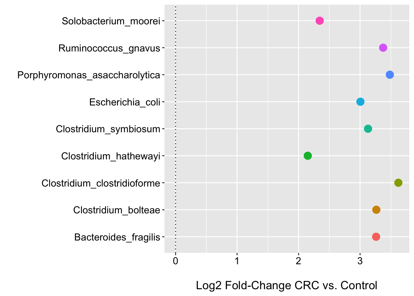
Here we see that no species has a low FDR p-value (even at < 0.25). This is where I would usually stop and/or perhaps focus on effect sizes etc.. However, for the purposes of illustration, we will look at those species with raw p-value < 0.05. We can see that there are nine species associated with CRC status and all have log2 fold changes > 2 for the point estimate (we could/should improve the plot by adding the 95% CIs…give it a go).
Maaslin2 also outputs residuals etc. for model diagnostic purposes. These might be worth looking at; however, we may not expect the residuals to be “all that well” normally distributed due to the excess zeros etc. At decent samples sizes this is not likely much of an issue unless the goal is to make predictions from the models. Heteroskedastic errors are more problematic given we are screening on the adjusted p-values. You may want to fit a few of these models using the base R lm function to quickly check that assumption and others (not sure if Maaslin2 outputs fitted values). All-in-all at this sample size the LM should give us a decent estimate for the conditional mean to help distinguish those taxa that look to be changing most in absolute abundance.
However, as an alternative, we can easily fit a more flexible compound Poisson linear model (CPLM) to these data…also known as the Tweedie model. This distribution will allows us to perhaps better model semi-continuous, positive data that contains a large probability mass at zero. We could also consider other approaches like Tobit regression or two-stage models (i.e., hurdle or mixture models), but this would change the quantity we are estimating (i.e., inference among those in which taxa is observed for the count/location parameter). Since the CPLM is an option in Maaslin2…lets give it a go!
m2_cplm <- Maaslin2(
  input_data = data.frame(otu_table(ps_norm)),
  input_metadata = data.frame(sample_data(ps_norm)),
  output = "/users/olljt2/desktop/wrench_rproj/mas_out/wrench_cplm",
  normalization = "NONE",
  transform = "NONE",
  analysis_method = "CPLM",
  fixed_effects = c("study_condition", "age", "gender", "BMI"),
  min_prevalence = 0.3,
  plot_heatmap = FALSE,
  plot_scatter = FALSE)
m2_cplm_df <- m2_cplm$results %>%
dplyr::filter(metadata == "study_condition") %>%
dplyr::select(-qval) %>%
dplyr::arrange(pval) %>%
dplyr::mutate(qval = p.adjust(pval, method = "fdr"))
(m2_cplm_fdr_df <- m2_cplm_df %>%
filter(qval < 0.25))## [1] feature metadata value coef stderr pval
## [7] name N N.not.zero qval
## <0 rows> (or 0-length row.names)(m2_cplm_pval_df <- m2_cplm_df %>%
filter(pval < 0.05)) %>%
dplyr::select(-name)## feature metadata value coef stderr
## 1 Porphyromonas_asaccharolytica study_condition CRC 0.8934917 0.32557683
## 2 Clostridium_bolteae study_condition CRC 0.2211337 0.08066320
## 3 Bacteroides_fragilis study_condition CRC 0.2141208 0.08542942
## 4 Clostridium_clostridioforme study_condition CRC 0.4691226 0.19962927
## 5 Ruminococcus_gnavus study_condition CRC 0.2609001 0.11236644
## 6 Escherichia_coli study_condition CRC 0.2243214 0.09733082
## 7 Clostridium_symbiosum study_condition CRC 0.2991218 0.13112178
## 8 Clostridium_hathewayi study_condition CRC 0.1732611 0.08439360
## 9 Solobacterium_moorei study_condition CRC 0.4453142 0.22260251
## pval N N.not.zero qval
## 1 0.007237274 101 34 0.5196150
## 2 0.007296483 101 91 0.5196150
## 3 0.013877710 101 91 0.5196150
## 4 0.020822379 101 55 0.5196150
## 5 0.022354018 101 83 0.5196150
## 6 0.023336190 101 87 0.5196150
## 7 0.024743570 101 74 0.5196150
## 8 0.042791896 101 90 0.7128421
## 9 0.048271829 101 49 0.7128421setdiff(m2_pval_df$feature, m2_cplm_pval_df$feature)## character(0)We can see that we get the same nine taxa with low p-values. If we look at the coefficients they look to be on the log scale (log-linear model). We could exponentiate these values if we wanted to compare them to the LM results. So we seem to be getting the same “general picture” for these data using either model.
Examining alternative normalization strategies via Maaslin2
Given the choice of the normalization strategy can be as, or more, important than the type of model selected for differential abundance testing, let’s fit a few other linear models available in Maaslin2 to see if we get similar results (and to serve as a code base for those interested in fitting other types of linear models in Maaslin2). One could also fit models to the scaled counts (i.e., NB, ZINB), but I do not do that here. I recommend taking a look at the performance of the various approaches in Maaslin2 in this recent pre-print.
Below I fit:
- The default approach (linear model on the log transformed relative abundances; total sum scaling [TSS] normalization)
- Maaslin1 default (linear model on the arcsin transformed relative abundances)
- Linear model to the centered log-ratio transformed values (pseudo count of 1 added to allow log-transform)
I could/should write a function that will fit each model and then do the FDR correction, but I want to keep the code here as simple as possible.
m2_def <- Maaslin2(
  input_data = data.frame(otu_table(ps)),
  input_metadata = data.frame(sample_data(ps)),
  output = "/users/olljt2/desktop/wrench_rproj/mas_out/tss",
  normalization = "TSS",
  transform = "LOG",
  analysis_method = "LM",
  fixed_effects = c("study_condition", "age", "gender", "BMI"),
  min_prevalence = 0.3,
  plot_heatmap = FALSE,
  plot_scatter = FALSE)

m2_arcsin <- Maaslin2(
  input_data = data.frame(otu_table(ps)),
  input_metadata = data.frame(sample_data(ps)),
  output = "/users/olljt2/desktop/wrench_rproj/mas_out/arcsin",
  normalization = "TSS",
  transform = "AST",
  analysis_method = "LM",
  fixed_effects = c("study_condition", "age", "gender", "BMI"),
  min_prevalence = 0.3,
  plot_heatmap = FALSE,
  plot_scatter = FALSE)

m2_clr <- Maaslin2(
  input_data = data.frame(otu_table(ps)),
  input_metadata = data.frame(sample_data(ps)),
  output = "/users/olljt2/desktop/wrench_rproj/mas_out/clr",
  normalization = "CLR",
  transform = "NONE",
  analysis_method = "LM",
  fixed_effects = c("study_condition", "age", "gender", "BMI"),
  min_prevalence = 0.3,
  plot_heatmap = FALSE,
  plot_scatter = FALSE)
m2_def_df <- m2_def$results %>%
dplyr::filter(metadata == "study_condition") %>%
dplyr::select(-qval) %>%
dplyr::arrange(pval) %>%
dplyr::mutate(qval = p.adjust(pval, method = "fdr"))
m2_arcsin_df <- m2_arcsin$results %>%
dplyr::filter(metadata == "study_condition") %>%
dplyr::select(-qval) %>%
dplyr::arrange(pval) %>%
dplyr::mutate(qval = p.adjust(pval, method = "fdr"))
m2_clr_df <- m2_clr$results %>%
dplyr::filter(metadata == "study_condition") %>%
dplyr::select(-qval) %>%
dplyr::arrange(pval) %>%
dplyr::mutate(qval = p.adjust(pval, method = "fdr"))
(m2_def_fdr_df <- m2_def_df %>% filter(qval < 0.25))## [1] feature metadata value coef stderr pval
## [7] name N N.not.zero qval
## <0 rows> (or 0-length row.names)(m2_arcsin_fdr_df <- m2_arcsin_df %>% filter(qval < 0.25))## [1] feature metadata value coef stderr pval
## [7] name N N.not.zero qval
## <0 rows> (or 0-length row.names)(m2_clr_fdr_df <- m2_clr_df %>% filter(qval < 0.25))## [1] feature metadata value coef stderr pval
## [7] name N N.not.zero qval
## <0 rows> (or 0-length row.names)m2_def_pval_df <- m2_def_df %>% filter(pval < 0.05)
m2_arcsin_pval_df <- m2_arcsin_df %>% filter(pval < 0.05)
m2_clr_pval_df <- m2_clr_df %>% filter(pval < 0.05)
da_venn <- venn.diagram(
x = list(m2_pval_df$feature, m2_def_pval_df$feature, m2_arcsin_pval_df$feature, m2_clr_pval_df$feature),
category.names = c("Wrench" , "TSS", "Arcsin", "CLR"),
filename = NULL,
fill = c("#8DD3C7", "#FFFFB3", "#BEBADA", "#FB8072"),
margin = 0.1)
grid::grid.newpage()
grid::grid.draw(da_venn) 
We can see that the results are generally similar in that none have low FDR p-values. This is good news with respect to the robustness of the results to the models selected. There is also a fair bit of overlap in those taxa identified with low raw p-values. Focusing on those called DA by three or more approaches (and with larger effect sizes and results not driven by a few outliers) might be a reasonable next step.
We can also plot the results so we can more clearly see which taxa overlap across approaches.
ggplot(m2_def_pval_df, aes(x = feature, y = coef, color = feature)) +
  geom_point(size = 4) +
  labs(y = "\nCRC vs. Control", x = "", shape = "") +
  theme(axis.text.x = element_text(color = "black", size = 12),
        axis.text.y = element_text(color = "black", size = 12),
        axis.title.y = element_text(size = 14),
        axis.title.x = element_text(size = 14),
        legend.text = element_text(size = 12),
        strip.text.x = element_text(size = 12, face = "bold"),
        legend.position = "bottom") +
  coord_flip() +
  guides(color = FALSE) +
  geom_hline(yintercept = 0, linetype="dotted")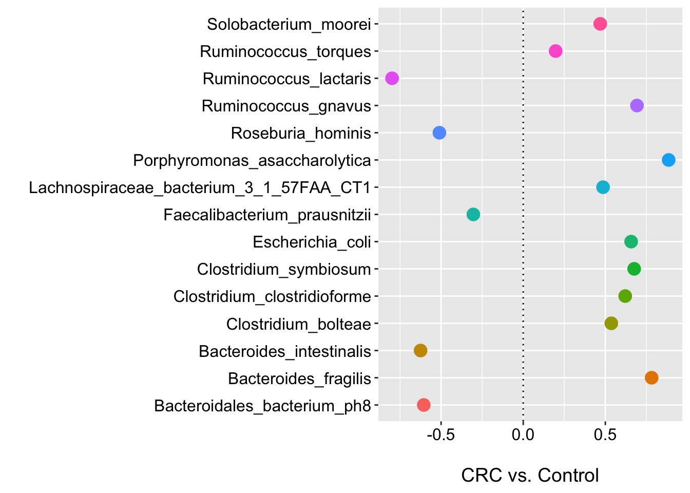
ggplot(m2_arcsin_pval_df, aes(x = feature, y = coef, color = feature)) +
  geom_point(size = 4) +
  labs(y = "\nCRC vs. Control", x = "", shape = "") +
  theme(axis.text.x = element_text(color = "black", size = 12),
        axis.text.y = element_text(color = "black", size = 12),
        axis.title.y = element_text(size = 14),
        axis.title.x = element_text(size = 14),
        legend.text = element_text(size = 12),
        strip.text.x = element_text(size = 12, face = "bold"),
        legend.position = "bottom") +
  coord_flip() +
  guides(color = FALSE) +
  geom_hline(yintercept = 0, linetype="dotted")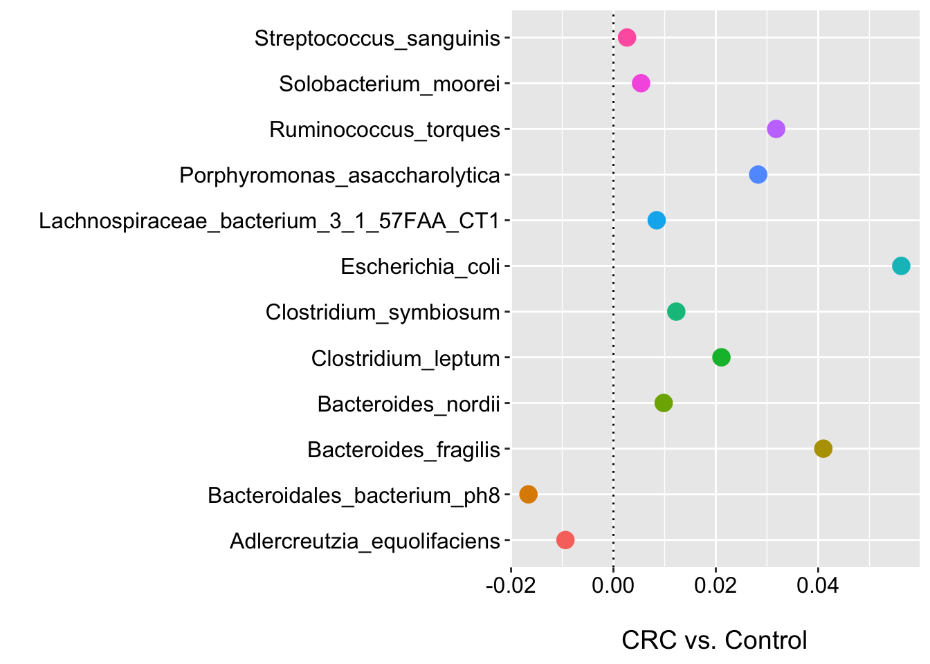
ggplot(m2_clr_pval_df, aes(x = feature, y = coef, color = feature)) +
  geom_point(size = 4) +
  labs(y = "\nCRC vs. Control", x = "", shape = "") +
  theme(axis.text.x = element_text(color = "black", size = 12),
        axis.text.y = element_text(color = "black", size = 12),
        axis.title.y = element_text(size = 14),
        axis.title.x = element_text(size = 14),
        legend.text = element_text(size = 12),
        strip.text.x = element_text(size = 12, face = "bold"),
        legend.position = "bottom") +
  coord_flip() +
  guides(color = FALSE) +
  geom_hline(yintercept = 0, linetype="dotted")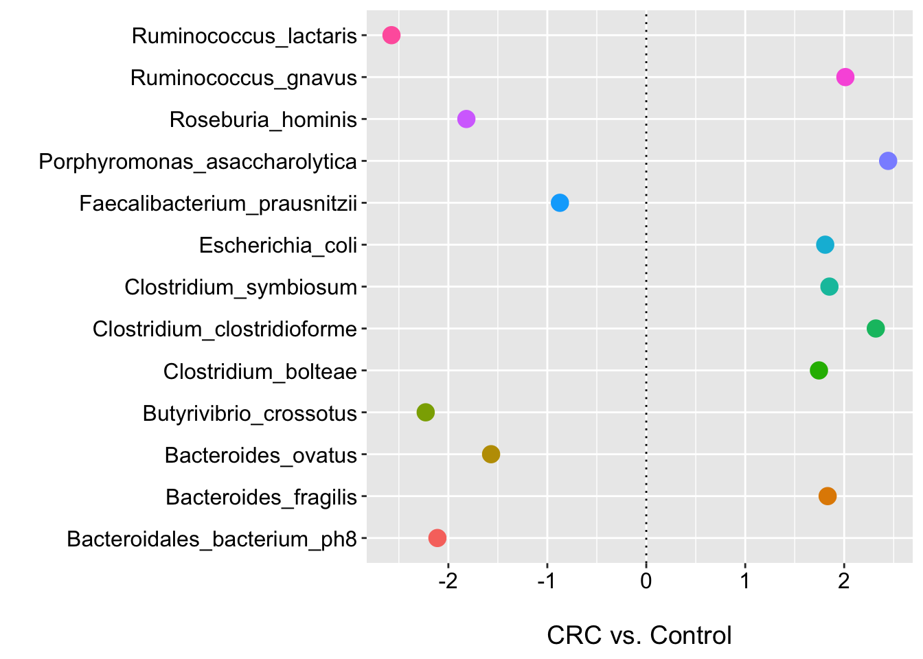
Wrench norm factors as model offsets
The norm factors obtained from the Wrench function can also be passed as offsets to many common DA tools like DESEq2, metagenomeSeq, edgeR, etc. Below I show how to pass the norm factors to DESeq2 and metagenomeSeq and then perform the DA testing. This approach is shown in the examples for the wrench function…so nothing new here…but wanted to include for completeness.
First, I filter the species based on their prevalence as we did above and then fit the models.
(ps_filt <- filter_taxa(ps, function(x) sum(x > 0) > (0.3*length(x)), TRUE))## phyloseq-class experiment-level object
## otu_table() OTU Table: [ 147 taxa and 101 samples ]
## sample_data() Sample Data: [ 101 samples by 18 sample variables ]
## tax_table() Taxonomy Table: [ 147 taxa by 8 taxonomic ranks ]dds <- phyloseq_to_deseq2(ps_filt, ~ study_condition + age + gender + BMI)
sizeFactors(dds) <- norm_factors
dds <- DESeq(dds, fitType = 'local')
res <- lfcShrink(dds, coef=2, type="apeglm")
deseq_res_df <- data.frame(res) %>%
rownames_to_column(var = "Species") %>%
dplyr::arrange(padj)
(fdr_deseq <- deseq_res_df %>%
dplyr::filter(padj < 0.25))## Species baseMean log2FoldChange lfcSE pvalue
## 1 Ruminococcus_torques 2920949 1.310603 0.5387872 0.0004265685
## padj
## 1 0.06270558(pval_deseq <- deseq_res_df %>%
dplyr::filter(pvalue < 0.05))## Species baseMean log2FoldChange lfcSE
## 1 Ruminococcus_torques 2920949.15 1.3106028 0.5387872
## 2 Faecalibacterium_prausnitzii 12826152.06 0.7276075 0.5533278
## 3 Eubacterium_rectale 9664692.51 0.8504668 0.6864710
## 4 Clostridium_asparagiforme 65685.45 0.4421056 0.5943626
## pvalue padj
## 1 0.0004265685 0.06270558
## 2 0.0163902240 0.80312098
## 3 0.0112887504 0.80312098
## 4 0.0401599309 0.99992317We get some similar hits using DESeq2 as we have seen in other models (actually a few less).
mseq_obj <- newMRexperiment(
  counts = data.frame(otu_table(ps_filt)),
  phenoData = AnnotatedDataFrame(data.frame(sample_data(ps_filt))),
)

normFactors(mseq_obj) <- norm_factors
pd <- pData(mseq_obj)
mod_matrix <- model.matrix(~ 1 + study_condition, data = pd)

mseq_res <- fitFeatureModel(mseq_obj, mod = mod_matrix)

mseq_df <- data.frame(MRcoefs(mseq_res, number = nrow(data.frame(otu_table(ps_filt)))))
mseq_df <- mseq_df %>%
  dplyr::arrange(adjPvalues)

(fdr_mseq <- mseq_df %>%
    dplyr::filter(adjPvalues < 0.25))
## logFC se pvalues
## Porphyromonas_asaccharolytica 3.540890 1.0218720 0.0005300306
## Bacteroides_fragilis 2.084528 0.6071855 0.0005967222
## Lachnospiraceae_bacterium_3_1_57FAA_CT1 1.711824 0.5472717 0.0017604547
## Clostridium_symbiosum 1.457101 0.4607562 0.0015646774
## Bacteroides_nordii 2.232524 0.7825436 0.0043321290
## Atopobium_parvulum 1.638123 0.5839742 0.0050296528
## Streptococcus_mitis_oralis_pneumoniae 1.579125 0.5480481 0.0039596097
## Escherichia_coli 1.555367 0.5830578 0.0076394607
## Lachnospiraceae_bacterium_2_1_58FAA 1.713594 0.6779548 0.0114847504
## Solobacterium_moorei 1.494695 0.6092467 0.0141532603
## Streptococcus_sanguinis 1.166811 0.5123147 0.0227547536
## Clostridium_bolteae 1.155491 0.5083018 0.0230118235
## Streptococcus_parasanguinis 1.019086 0.4482367 0.0229933478
## Clostridium_leptum 0.949567 0.4164069 0.0225850085
## adjPvalues
## Porphyromonas_asaccharolytica 0.04385908
## Bacteroides_fragilis 0.04385908
## Lachnospiraceae_bacterium_3_1_57FAA_CT1 0.06469671
## Clostridium_symbiosum 0.06469671
## Bacteroides_nordii 0.10562271
## Atopobium_parvulum 0.10562271
## Streptococcus_mitis_oralis_pneumoniae 0.10562271
## Escherichia_coli 0.14037509
## Lachnospiraceae_bacterium_2_1_58FAA 0.18758426
## Solobacterium_moorei 0.20805293
## Streptococcus_sanguinis 0.24162415
## Clostridium_bolteae 0.24162415
## Streptococcus_parasanguinis 0.24162415
## Clostridium_leptum 0.24162415(pval_mseq <- mseq_df %>%
dplyr::filter(pvalues < 0.05))## logFC se pvalues
## Porphyromonas_asaccharolytica 3.5408905 1.0218720 0.0005300306
## Bacteroides_fragilis 2.0845285 0.6071855 0.0005967222
## Lachnospiraceae_bacterium_3_1_57FAA_CT1 1.7118244 0.5472717 0.0017604547
## Clostridium_symbiosum 1.4571011 0.4607562 0.0015646774
## Bacteroides_nordii 2.2325242 0.7825436 0.0043321290
## Atopobium_parvulum 1.6381226 0.5839742 0.0050296528
## Streptococcus_mitis_oralis_pneumoniae 1.5791247 0.5480481 0.0039596097
## Escherichia_coli 1.5553665 0.5830578 0.0076394607
## Lachnospiraceae_bacterium_2_1_58FAA 1.7135935 0.6779548 0.0114847504
## Solobacterium_moorei 1.4946954 0.6092467 0.0141532603
## Streptococcus_sanguinis 1.1668108 0.5123147 0.0227547536
## Clostridium_bolteae 1.1554911 0.5083018 0.0230118235
## Streptococcus_parasanguinis 1.0190864 0.4482367 0.0229933478
## Clostridium_leptum 0.9495670 0.4164069 0.0225850085
## Ruminococcus_gnavus 1.3741782 0.6537046 0.0355410713
## Eggerthella_unclassified 0.9595872 0.4707206 0.0414950288
## Clostridiales_bacterium_1_7_47FAA 0.9304408 0.4695931 0.0475490757
## adjPvalues
## Porphyromonas_asaccharolytica 0.04385908
## Bacteroides_fragilis 0.04385908
## Lachnospiraceae_bacterium_3_1_57FAA_CT1 0.06469671
## Clostridium_symbiosum 0.06469671
## Bacteroides_nordii 0.10562271
## Atopobium_parvulum 0.10562271
## Streptococcus_mitis_oralis_pneumoniae 0.10562271
## Escherichia_coli 0.14037509
## Lachnospiraceae_bacterium_2_1_58FAA 0.18758426
## Solobacterium_moorei 0.20805293
## Streptococcus_sanguinis 0.24162415
## Clostridium_bolteae 0.24162415
## Streptococcus_parasanguinis 0.24162415
## Clostridium_leptum 0.24162415
## Ruminococcus_gnavus 0.34830250
## Eggerthella_unclassified 0.38123558
## Clostridiales_bacterium_1_7_47FAA 0.40970005For metagenomeSeq we actually see a few species with low FDR p-values (many also have low raw p-values in other models). However, these results are not adjusted for age, gender and BMI. Covariate adjustment in these examples is included primarily for didactic purposes, but I do recommend thoughtful selection regarding covariate inclusion given the literature (at the time of writing) suggests the microbiome may be associated with many exposures and outcomes of interest, but is remains unclear as to how much of this might be causal.
At the time of writing this, it does not look like the fitFeatureModel (i.e., zero-inflated log normal) model is able to handle covariates. I look forward to any thoughts on whether this is not the case, but if true, makes this approach much more limited for applied use.
Bonus: GMPR normalization
Here I include some short code for another normalization approach I use often that is designed specifically for sparse microbiome data. The geometric mean of pairwise ratios (GMPR) method as stated by the authors was developed for the unique characteristics of microbiome data, which contain a vast number of zeros due to the physical absence or under-sampling of microbes.
The approach is described here and the function is available here on GitHub.
The function expects features as columns and subjects as rows.
These norm factors could also be dropped into the workflows above.
count_tab_gmpr <- data.frame(t(as.matrix(data.frame(otu_table(ps)))))
gmpr_norm_factors <- GMPR(count_tab_gmpr)
head(gmpr_norm_factors)
## MMRS11288076ST MMRS11932626ST MMRS12272136ST MMRS14379078ST MMRS15137911ST
## 1.2286534 1.1922496 1.0353900 0.9520517 1.4351891
## MMRS16644320ST
## 1.4954715Session Info
sessionInfo()## R version 4.0.4 (2021-02-15)
## Platform: x86_64-apple-darwin17.0 (64-bit)
## Running under: macOS Catalina 10.15.7
##
## Matrix products: default
## BLAS: /Library/Frameworks/R.framework/Versions/4.0/Resources/lib/libRblas.dylib
## LAPACK: /Library/Frameworks/R.framework/Versions/4.0/Resources/lib/libRlapack.dylib
##
## locale:
## [1] en_US.UTF-8/en_US.UTF-8/en_US.UTF-8/C/en_US.UTF-8/en_US.UTF-8
##
## attached base packages:
## [1] grid stats4 parallel stats graphics grDevices utils
## [8] datasets methods base
##
## other attached packages:
## [1] GMPR_0.1.3 metagenomeSeq_1.30.0
## [3] RColorBrewer_1.1-2 glmnet_4.0-2
## [5] Matrix_1.3-2 limma_3.44.3
## [7] VennDiagram_1.6.20 futile.logger_1.4.3
## [9] DescTools_0.99.38 Maaslin2_1.2.0
## [11] Wrench_1.8.0 apeglm_1.10.0
## [13] DESeq2_1.28.1 SummarizedExperiment_1.18.2
## [15] DelayedArray_0.14.1 matrixStats_0.57.0
## [17] GenomicRanges_1.40.0 GenomeInfoDb_1.24.2
## [19] IRanges_2.22.2 S4Vectors_0.26.1
## [21] phyloseq_1.32.0 forcats_0.5.0
## [23] stringr_1.4.0 purrr_0.3.4
## [25] readr_1.3.1 tidyr_1.1.2
## [27] tibble_3.0.3 ggplot2_3.3.2
## [29] tidyverse_1.3.0 curatedMetagenomicData_1.18.2
## [31] ExperimentHub_1.14.2 dplyr_1.0.2
## [33] Biobase_2.48.0 AnnotationHub_2.20.2
## [35] BiocFileCache_1.12.1 dbplyr_1.4.4
## [37] BiocGenerics_0.34.0
##
## loaded via a namespace (and not attached):
## [1] tidyselect_1.1.0 tweedie_2.3.2
## [3] RSQLite_2.2.0 AnnotationDbi_1.50.3
## [5] BiocParallel_1.22.0 munsell_0.5.0
## [7] codetools_0.2-18 statmod_1.4.34
## [9] withr_2.2.0 colorspace_1.4-1
## [11] knitr_1.30 rstudioapi_0.11
## [13] robustbase_0.93-6 lars_1.2
## [15] labeling_0.3 optparse_1.6.6
## [17] bbmle_1.0.23.1 GenomeInfoDbData_1.2.3
## [19] lpsymphony_1.16.0 farver_2.0.3
## [21] bit64_4.0.5 rhdf5_2.32.2
## [23] coda_0.19-4 vctrs_0.3.4
## [25] generics_0.0.2 lambda.r_1.2.4
## [27] xfun_0.19 R6_2.5.0
## [29] locfit_1.5-9.4 chemometrics_1.4.2
## [31] bitops_1.0-6 assertthat_0.2.1
## [33] promises_1.1.1 scales_1.1.1
## [35] nnet_7.3-15 rootSolve_1.8.2.1
## [37] gtable_0.3.0 lmom_2.8
## [39] rlang_0.4.8 genefilter_1.70.0
## [41] splines_4.0.4 broom_0.7.0
## [43] BiocManager_1.30.10 yaml_2.2.1
## [45] reshape2_1.4.4 modelr_0.1.8
## [47] backports_1.1.9 httpuv_1.5.4
## [49] tools_4.0.4 bookdown_0.21
## [51] logging_0.10-108 ellipsis_0.3.1
## [53] gplots_3.1.0 biomformat_1.16.0
## [55] Rcpp_1.0.5 hash_2.2.6.1
## [57] plyr_1.8.6 zlibbioc_1.34.0
## [59] RCurl_1.98-1.2 rpart_4.1-15
## [61] pbapply_1.4-3 haven_2.3.1
## [63] cluster_2.1.0 fs_1.5.0
## [65] magrittr_2.0.1 data.table_1.13.0
## [67] futile.options_1.0.1 blogdown_0.21.45
## [69] reprex_0.3.0 mvtnorm_1.1-1
## [71] cplm_0.7-9 hms_0.5.3
## [73] mime_0.9 evaluate_0.14
## [75] xtable_1.8-4 XML_3.99-0.5
## [77] emdbook_1.3.12 mclust_5.4.6
## [79] readxl_1.3.1 shape_1.4.5
## [81] compiler_4.0.4 bdsmatrix_1.3-4
## [83] KernSmooth_2.23-18 crayon_1.3.4
## [85] minqa_1.2.4 htmltools_0.5.0
## [87] mgcv_1.8-33 pcaPP_1.9-73
## [89] later_1.1.0.1 geneplotter_1.66.0
## [91] expm_0.999-5 Exact_2.1
## [93] lubridate_1.7.9 DBI_1.1.0
## [95] formatR_1.7 biglm_0.9-2
## [97] MASS_7.3-53 rappdirs_0.3.1
## [99] boot_1.3-26 som_0.3-5.1
## [101] ade4_1.7-15 getopt_1.20.3
## [103] permute_0.9-5 cli_2.0.2
## [105] igraph_1.2.5 pkgconfig_2.0.3
## [107] numDeriv_2016.8-1.1 xml2_1.3.2
## [109] foreach_1.5.0 annotate_1.66.0
## [111] multtest_2.44.0 XVector_0.28.0
## [113] rvest_0.3.6 digest_0.6.27
## [115] pls_2.7-3 vegan_2.5-6
## [117] Biostrings_2.56.0 rmarkdown_2.5
## [119] cellranger_1.1.0 gld_2.6.2
## [121] curl_4.3 shiny_1.5.0
## [123] gtools_3.8.2 lifecycle_0.2.0
## [125] nlme_3.1-152 jsonlite_1.7.1
## [127] Rhdf5lib_1.10.1 fansi_0.4.1
## [129] pillar_1.4.6 lattice_0.20-41
## [131] fastmap_1.0.1 httr_1.4.2
## [133] DEoptimR_1.0-8 survival_3.2-7
## [135] interactiveDisplayBase_1.26.3 glue_1.4.2
## [137] iterators_1.0.12 BiocVersion_3.11.1
## [139] bit_4.0.4 class_7.3-18
## [141] stringi_1.5.3 blob_1.2.1
## [143] caTools_1.18.0 memoise_1.1.0
## [145] e1071_1.7-3 ape_5.4-1