Introduction to Phyloseq
This post is from a tutorial demonstrating the processing of amplicon short read data in R taught as part of the Introduction to Metagenomics Summer Workshop. It provides a quick introduction some of the functionality provided by phyloseq and follows some of Paul McMurdie’s excellent tutorials. This tutorial picks up where Ben Callahan’s DADA2 tutorial leaves off and highlights some of the main accessor and processor functions of the package. I thought it might be useful to a broader audience so decided to post it.
The goal of this interactive session is to introduce you to some of the basic functionality of the phyloseq package that can help you to explore and better understand your metagenomic data. We will be working with the phyloseq object that was created during the DADA2 tutorial. If you recall, these were murine stool samples collected from a single mouse over time. The phyloseq object contains: an ASV table, sample metadata, taxonomic classifications, and the reference sequences. We did not generate a phylogenetic tree from these sequences, but if we had, it could be included as well.
The session will quickly cover some of the basic accessor, analysis and graphical functions available to you when using the phyloseq package in R.
To learn more, Paul McMurdie has an excellent set of tutorials that I encourage you to explore.
Loading required packages and phyloseq object
library(dada2); packageVersion("dada2") ## Loading required package: Rcpp## [1] '1.12.1'library(phyloseq); packageVersion("phyloseq") ## [1] '1.28.0'library(ggplot2); packageVersion("ggplot2") ## [1] '3.2.0'If the phyloseq (ps) object is not already loaded into your environment…let’s go ahead and do that now. You will need to change the path so that it maps to the ps object on your computer. No path is needed if you are working in an RStudio project folder (or if you cloned the folder from GitHub).
ps <- readRDS("C:/Users/olljt2/Desktop/academic_web_page/static/data/ps.rds")Accessing the sample information and sample metadata
ps## phyloseq-class experiment-level object
## otu_table() OTU Table: [ 232 taxa and 19 samples ]
## sample_data() Sample Data: [ 19 samples by 4 sample variables ]
## tax_table() Taxonomy Table: [ 232 taxa by 7 taxonomic ranks ]
## refseq() DNAStringSet: [ 232 reference sequences ]- Here we can see that we have a phyloseq object that consists of:
- An OTU table with 232 taxa and 19 samples
- A sample metadata file consisting of 4 variables
- A taxonomy table with 7 ranks
- Reference sequences on all 232 taxa
This highlights one of the key advantages of working with phyloseq objects in R. Each of these data structures is contained in a single object. This makes it easy to keep all of your data together and to share it with colleagues or include it as a supplemental file to a publication.
Next we will see how each of the components can be accessed. We will run through several commands below and then discuss the output.
nsamples(ps)## [1] 19sample_names(ps)## [1] "F3D0" "F3D1" "F3D141" "F3D142" "F3D143" "F3D144" "F3D145"
## [8] "F3D146" "F3D147" "F3D148" "F3D149" "F3D150" "F3D2" "F3D3"
## [15] "F3D5" "F3D6" "F3D7" "F3D8" "F3D9"sample_variables(ps)## [1] "Subject" "Gender" "Day" "When"head(sample_data(ps))## Subject Gender Day When
## F3D0 3 F 0 Early
## F3D1 3 F 1 Early
## F3D141 3 F 141 Late
## F3D142 3 F 142 Late
## F3D143 3 F 143 Late
## F3D144 3 F 144 Latesample_data(ps)$When## [1] "Early" "Early" "Late" "Late" "Late" "Late" "Late" "Late"
## [9] "Late" "Late" "Late" "Late" "Early" "Early" "Early" "Early"
## [17] "Early" "Early" "Early"table(sample_data(ps)$When)##
## Early Late
## 9 10median(sample_data(ps)$Day)## [1] 141metadata <- data.frame(sample_data(ps))
head(metadata)## Subject Gender Day When
## F3D0 3 F 0 Early
## F3D1 3 F 1 Early
## F3D141 3 F 141 Late
## F3D142 3 F 142 Late
## F3D143 3 F 143 Late
## F3D144 3 F 144 LateHere we can see that we have 19 samples and they are assigned the sample names we gave them during the DADA2 tutorial. We also have 4 variables (Subject, Gender, Day, and When) and that information can be easily accessed and computations or descriptive statistics performed. Specific components of the ps object can be extracted and converted to a data.frame for additional analyses.
Examining the number of reads for each sample
Phyloseq makes it easy to calculate the total number of reads for each sample, sort them to identify potentially problematic samples, and plot their distribution.
sample_sums(ps)## F3D0 F3D1 F3D141 F3D142 F3D143 F3D144 F3D145 F3D146 F3D147 F3D148
## 6528 5017 4863 2521 2518 3488 5820 3879 13006 9935
## F3D149 F3D150 F3D2 F3D3 F3D5 F3D6 F3D7 F3D8 F3D9
## 10653 4240 16835 5491 3716 6679 4217 4547 6015sort(sample_sums(ps))## F3D143 F3D142 F3D144 F3D5 F3D146 F3D7 F3D150 F3D8 F3D141 F3D1
## 2518 2521 3488 3716 3879 4217 4240 4547 4863 5017
## F3D3 F3D145 F3D9 F3D0 F3D6 F3D148 F3D149 F3D147 F3D2
## 5491 5820 6015 6528 6679 9935 10653 13006 16835hist(sample_sums(ps), main="Histogram: Read Counts", xlab="Total Reads",
border="blue", col="green", las=1, breaks=12)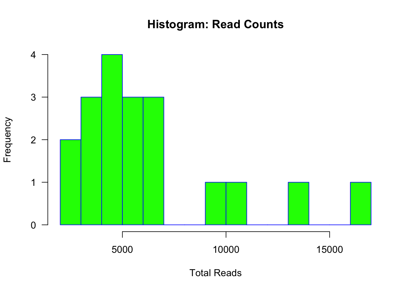
metadata$total_reads <- sample_sums(ps)Here we see that the number of reads per sample ranges from 2,518 to 16,835 and most samples have less than 10k reads. Try to calculate the mean and median number of reads on your own.
The last line of code above can be used to add a new column containing the total read count to the metadata data.frame. Similarly, sample_data(ps)$total_reads <- sample_sums(ps) would add this information to the phyloseq object itself (as a new sample_data variable).
Examining the OTU table
ntaxa(ps)## [1] 232head(taxa_names(ps))## [1] "ASV1" "ASV2" "ASV3" "ASV4" "ASV5" "ASV6"head(taxa_sums(ps))## ASV1 ASV2 ASV3 ASV4 ASV5 ASV6
## 14148 9898 8862 7935 5880 5469(asv_tab <- data.frame(otu_table(ps)[1:5, 1:5]))## ASV1 ASV2 ASV3 ASV4 ASV5
## F3D0 579 345 449 430 154
## F3D1 405 353 231 69 140
## F3D141 444 362 345 502 189
## F3D142 289 304 158 164 180
## F3D143 228 176 204 231 130- Phyloseq allows you to easily:
- Obtain a count of the number of taxa
- Access their names (e.g. ASV1, ASV2, …)
- Get a count of each ASV summed over all samples
- Extract the OTU table as a data.frame
Examining the taxonomy
rank_names(ps)## [1] "Kingdom" "Phylum" "Class" "Order" "Family" "Genus" "Species"head(tax_table(ps))## Taxonomy Table: [6 taxa by 7 taxonomic ranks]:
## Kingdom Phylum Class Order
## ASV1 "Bacteria" "Bacteroidetes" "Bacteroidia" "Bacteroidales"
## ASV2 "Bacteria" "Bacteroidetes" "Bacteroidia" "Bacteroidales"
## ASV3 "Bacteria" "Bacteroidetes" "Bacteroidia" "Bacteroidales"
## ASV4 "Bacteria" "Bacteroidetes" "Bacteroidia" "Bacteroidales"
## ASV5 "Bacteria" "Bacteroidetes" "Bacteroidia" "Bacteroidales"
## ASV6 "Bacteria" "Bacteroidetes" "Bacteroidia" "Bacteroidales"
## Family Genus Species
## ASV1 "Muribaculaceae" NA NA
## ASV2 "Muribaculaceae" NA NA
## ASV3 "Muribaculaceae" NA NA
## ASV4 "Muribaculaceae" NA NA
## ASV5 "Bacteroidaceae" "Bacteroides" NA
## ASV6 "Muribaculaceae" NA NAhead(tax_table(ps)[, 2])## Taxonomy Table: [6 taxa by 1 taxonomic ranks]:
## Phylum
## ASV1 "Bacteroidetes"
## ASV2 "Bacteroidetes"
## ASV3 "Bacteroidetes"
## ASV4 "Bacteroidetes"
## ASV5 "Bacteroidetes"
## ASV6 "Bacteroidetes"table(tax_table(ps)[, 2])##
## Actinobacteria Bacteroidetes Cyanobacteria
## 6 20 3
## Deinococcus-Thermus Epsilonbacteraeota Firmicutes
## 1 1 185
## Patescibacteria Proteobacteria Tenericutes
## 2 7 6
## Verrucomicrobia
## 1(tax_tab <- data.frame(tax_table(ps)[50:55, ]))## Kingdom Phylum Class Order
## ASV50 Bacteria Firmicutes Clostridia Clostridiales
## ASV51 Bacteria Firmicutes Clostridia Clostridiales
## ASV52 Bacteria Firmicutes Clostridia Clostridiales
## ASV53 Bacteria Epsilonbacteraeota Campylobacteria Campylobacterales
## ASV54 Bacteria Firmicutes Clostridia Clostridiales
## ASV55 Bacteria Firmicutes Clostridia Clostridiales
## Family Genus Species
## ASV50 Lachnospiraceae Acetatifactor <NA>
## ASV51 Ruminococcaceae Ruminiclostridium_5 <NA>
## ASV52 Lachnospiraceae Lachnospiraceae_UCG-001 <NA>
## ASV53 Helicobacteraceae Helicobacter pylori
## ASV54 Family_XIII <NA> <NA>
## ASV55 Ruminococcaceae Ruminiclostridium_5 <NA>Here we can see that we have information on 7 taxonomic ranks from Kingdom to Species. We can easily access specific components of this object to learn more about the classifications. For example, we see that the vast majority of ASVs are classified as Firmicutes. This is in line with our expectations. Conducting such assessments may help you identify potential sequencing errors that made it through the denoising pipeline (i.e. those not assigned to a Kingdom) or to understand the proportion of sequences classified at lower levels (i.e. genus or species).
One could also swap out this taxonomy file for another…say using the IDTAXA function in the DECIPHER package or an alternative reference database (i.e. Silva or Greengenes). I will let you look into this on your own!
Examining the reference sequences
Storing the reference sequences with your phyloseq object is critical of you rename the ASV names to ASV1, ASV2, … This will allow you to communicate the information on these ASVs directly (i.e. you can provide the exact sequence variant information). This information is also required to build a phylogenetic tree or BLAST the sequences against the NCBI database for example. In short, always include these in the phyloseq object.
Below we see that these sequences are stored as a DNAStringSet. The refseq command returns the ASV number, sequence length, and amplicon sequence for each ASV. The function dada2::nwhamming is calculating the Hamming distance of two sequences after alignment. We will discuss more about this in class. We can also pull out the component and store it as a data.frame.
head(refseq(ps))## A DNAStringSet instance of length 6
## width seq names
## [1] 252 TACGGAGGATGCGAGCGTTAT...AAGTGTGGGTATCGAACAGG ASV1
## [2] 252 TACGGAGGATGCGAGCGTTAT...AAGCGTGGGTATCGAACAGG ASV2
## [3] 252 TACGGAGGATGCGAGCGTTAT...AAGCGTGGGTATCGAACAGG ASV3
## [4] 252 TACGGAGGATGCGAGCGTTAT...AAGTGCGGGGATCGAACAGG ASV4
## [5] 253 TACGGAGGATCCGAGCGTTAT...AAGTGTGGGTATCAAACAGG ASV5
## [6] 252 TACGGAGGATGCGAGCGTTAT...AAGTGCGGGGATCAAACAGG ASV6dada2::nwhamming(as.vector(refseq(ps)[1]), as.vector(refseq(ps)[2]))## [1] 20(ref_tab <- data.frame(head(refseq(ps))))## head.refseq.ps..
## ASV1 TACGGAGGATGCGAGCGTTATCCGGATTTATTGGGTTTAAAGGGTGCGCAGGCGGAAGATCAAGTCAGCGGTAAAATTGAGAGGCTCAACCTCTTCGAGCCGTTGAAACTGGTTTTCTTGAGTGAGCGAGAAGTATGCGGAATGCGTGGTGTAGCGGTGAAATGCATAGATATCACGCAGAACTCCGATTGCGAAGGCAGCATACCGGCGCTCAACTGACGCTCATGCACGAAAGTGTGGGTATCGAACAGG
## ASV2 TACGGAGGATGCGAGCGTTATCCGGATTTATTGGGTTTAAAGGGTGCGCAGGCGGACTCTCAAGTCAGCGGTCAAATCGCGGGGCTCAACCCCGTTCCGCCGTTGAAACTGGGAGCCTTGAGTGCGCGAGAAGTAGGCGGAATGCGTGGTGTAGCGGTGAAATGCATAGATATCACGCAGAACTCCGATTGCGAAGGCAGCCTACCGGCGCGCAACTGACGCTCATGCACGAAAGCGTGGGTATCGAACAGG
## ASV3 TACGGAGGATGCGAGCGTTATCCGGATTTATTGGGTTTAAAGGGTGCGTAGGCGGGCTGTTAAGTCAGCGGTCAAATGTCGGGGCTCAACCCCGGCCTGCCGTTGAAACTGGCGGCCTCGAGTGGGCGAGAAGTATGCGGAATGCGTGGTGTAGCGGTGAAATGCATAGATATCACGCAGAACTCCGATTGCGAAGGCAGCATACCGGCGCCCGACTGACGCTGAGGCACGAAAGCGTGGGTATCGAACAGG
## ASV4 TACGGAGGATGCGAGCGTTATCCGGATTTATTGGGTTTAAAGGGTGCGTAGGCGGGCTTTTAAGTCAGCGGTAAAAATTCGGGGCTCAACCCCGTCCGGCCGTTGAAACTGGGGGCCTTGAGTGGGCGAGAAGAAGGCGGAATGCGTGGTGTAGCGGTGAAATGCATAGATATCACGCAGAACCCCGATTGCGAAGGCAGCCTTCCGGCGCCCTACTGACGCTGAGGCACGAAAGTGCGGGGATCGAACAGG
## ASV5 TACGGAGGATCCGAGCGTTATCCGGATTTATTGGGTTTAAAGGGAGCGTAGGTGGATTGTTAAGTCAGTTGTGAAAGTTTGCGGCTCAACCGTAAAATTGCAGTTGAAACTGGCAGTCTTGAGTACAGTAGAGGTGGGCGGAATTCGTGGTGTAGCGGTGAAATGCTTAGATATCACGAAGAACTCCGATTGCGAAGGCAGCTCACTGGACTGCAACTGACACTGATGCTCGAAAGTGTGGGTATCAAACAGG
## ASV6 TACGGAGGATGCGAGCGTTATCCGGATTTATTGGGTTTAAAGGGTGCGTAGGCGGCCTGCCAAGTCAGCGGTAAAATTGCGGGGCTCAACCCCGTACAGCCGTTGAAACTGCCGGGCTCGAGTGGGCGAGAAGTATGCGGAATGCGTGGTGTAGCGGTGAAATGCATAGATATCACGCAGAACCCCGATTGCGAAGGCAGCATACCGGCGCCCTACTGACGCTGAGGCACGAAAGTGCGGGGATCAAACAGGAccessing the phylogenetic tree
We did not generate a phylogenetic tree during the DADA2 tutorial in the interest of time. However, phyloseq has many excellent tools for working with and visualizing trees. I recommend you take a look at these tutorials below for some examples.
- https://joey711.github.io/phyloseq/preprocess.html
- https://joey711.github.io/phyloseq/plot_tree-examples.html
Ben Callahan’s F1000 paper demonstrates a complete analysis workflow in R including the construction of a de-novo phylogenetic tree. I highly recommned you take a look at this paper.
Agglomerating and subsetting taxa
Often times we may want to agglomerate taxa to a specific taxonomic rank for analysis. Or we may want to work with a given subset of taxa. We can perform these operations in phyloseq with the tax_glom and subset_taxa functions.
(ps_phylum <- tax_glom(ps, "Phylum"))## phyloseq-class experiment-level object
## otu_table() OTU Table: [ 10 taxa and 19 samples ]
## sample_data() Sample Data: [ 19 samples by 4 sample variables ]
## tax_table() Taxonomy Table: [ 10 taxa by 7 taxonomic ranks ]
## refseq() DNAStringSet: [ 10 reference sequences ]taxa_names(ps_phylum)## [1] "ASV1" "ASV11" "ASV19" "ASV53" "ASV67" "ASV90" "ASV107"
## [8] "ASV109" "ASV189" "ASV191"taxa_names(ps_phylum) <- tax_table(ps_phylum)[, 2]
taxa_names(ps_phylum)## [1] "Bacteroidetes" "Firmicutes" "Tenericutes"
## [4] "Epsilonbacteraeota" "Actinobacteria" "Patescibacteria"
## [7] "Proteobacteria" "Deinococcus-Thermus" "Cyanobacteria"
## [10] "Verrucomicrobia"otu_table(ps_phylum)[1:5, c(1:3, 5, 7)]## OTU Table: [5 taxa and 5 samples]
## taxa are columns
## Bacteroidetes Firmicutes Tenericutes Actinobacteria Proteobacteria
## F3D0 3708 2620 151 27 12
## F3D1 1799 3011 157 3 16
## F3D141 3437 1370 35 16 0
## F3D142 2003 452 33 28 0
## F3D143 1816 655 34 10 0Here we are agglomerating the counts to the Phylum-level and then renaming the ASVs to make them more descriptive. We can see that we have 10 Phyla. The ASV information (i.e. refseq and taxonomy for one of the ASVs in each Phylum) gets carried along for the ride (we can typically ignore this or you can remove these components if you prefer).
We can also subset taxa…
(ps_bacteroides <- subset_taxa(ps, Genus == "Bacteroides"))## phyloseq-class experiment-level object
## otu_table() OTU Table: [ 3 taxa and 19 samples ]
## sample_data() Sample Data: [ 19 samples by 4 sample variables ]
## tax_table() Taxonomy Table: [ 3 taxa by 7 taxonomic ranks ]
## refseq() DNAStringSet: [ 3 reference sequences ]tax_table(ps_bacteroides)## Taxonomy Table: [3 taxa by 7 taxonomic ranks]:
## Kingdom Phylum Class Order
## ASV5 "Bacteria" "Bacteroidetes" "Bacteroidia" "Bacteroidales"
## ASV80 "Bacteria" "Bacteroidetes" "Bacteroidia" "Bacteroidales"
## ASV163 "Bacteria" "Bacteroidetes" "Bacteroidia" "Bacteroidales"
## Family Genus Species
## ASV5 "Bacteroidaceae" "Bacteroides" NA
## ASV80 "Bacteroidaceae" "Bacteroides" "vulgatus"
## ASV163 "Bacteroidaceae" "Bacteroides" "vulgatus"prune_taxa(taxa_sums(ps) > 100, ps) ## phyloseq-class experiment-level object
## otu_table() OTU Table: [ 99 taxa and 19 samples ]
## sample_data() Sample Data: [ 19 samples by 4 sample variables ]
## tax_table() Taxonomy Table: [ 99 taxa by 7 taxonomic ranks ]
## refseq() DNAStringSet: [ 99 reference sequences ]filter_taxa(ps, function(x) sum(x > 10) > (0.1*length(x)), TRUE) ## phyloseq-class experiment-level object
## otu_table() OTU Table: [ 135 taxa and 19 samples ]
## sample_data() Sample Data: [ 19 samples by 4 sample variables ]
## tax_table() Taxonomy Table: [ 135 taxa by 7 taxonomic ranks ]
## refseq() DNAStringSet: [ 135 reference sequences ]- With the above commands we can quickly see that we have:
- A total of 3 ASVs classified as Bacteroides
- A total of 99 ASVs seen at least 100 times across all samples
- A total of 135 taxa seen at least 10 times in at least 10% of samples
This highlights how we might use phyloseq as a tool to filter taxa prior to statistical analysis.
Subsetting samples and tranforming counts
Phyloseq can also be used to subset all the individual components based on sample metadata information. This would take a fair bit of work to do properly if we were working with each individual component…and not with phyloseq. Below we subset the early stool samples. Then we generate an object that includes only samples with > 5,000 total reads.
ps_early <- subset_samples(ps, When == "Early")
(ps_early = prune_taxa(taxa_sums(ps_early) > 0, ps_early))
## phyloseq-class experiment-level object
## otu_table() OTU Table: [ 183 taxa and 9 samples ]
## sample_data() Sample Data: [ 9 samples by 4 sample variables ]
## tax_table() Taxonomy Table: [ 183 taxa by 7 taxonomic ranks ]
## refseq() DNAStringSet: [ 183 reference sequences ]sample_data(ps_early)$When## [1] "Early" "Early" "Early" "Early" "Early" "Early" "Early" "Early" "Early"sort(sample_sums(ps))## F3D143 F3D142 F3D144 F3D5 F3D146 F3D7 F3D150 F3D8 F3D141 F3D1
## 2518 2521 3488 3716 3879 4217 4240 4547 4863 5017
## F3D3 F3D145 F3D9 F3D0 F3D6 F3D148 F3D149 F3D147 F3D2
## 5491 5820 6015 6528 6679 9935 10653 13006 16835(ps_reads_GT_5k = prune_samples(sample_sums(ps) > 5000, ps))## phyloseq-class experiment-level object
## otu_table() OTU Table: [ 232 taxa and 10 samples ]
## sample_data() Sample Data: [ 10 samples by 4 sample variables ]
## tax_table() Taxonomy Table: [ 232 taxa by 7 taxonomic ranks ]
## refseq() DNAStringSet: [ 232 reference sequences ]sort(sample_sums(ps_reads_GT_5k))## F3D1 F3D3 F3D145 F3D9 F3D0 F3D6 F3D148 F3D149 F3D147 F3D2
## 5017 5491 5820 6015 6528 6679 9935 10653 13006 16835Counts can be converted to relative abundances (e.g. total sum scaling) using the transform_sample_counts function. They can also be subsampled/rarified using the rarefy_even_depth function. However, subsampling to account for differences in sequencing depth acorss samples has important limitations. See the papers below for a more in-depth discussion.
- McMurdie and Holmes, Waste Not, Want Not: Why Rarefying Microbiome Data Is Inadmissible
- Weiss et. al., Normalization and microbial differential abundance strategies depend upon data characteristics
ps_relabund <- transform_sample_counts(ps, function(x) x / sum(x))
otu_table(ps_relabund)[1:5, 1:5]
## OTU Table: [5 taxa and 5 samples]
## taxa are columns
## ASV1 ASV2 ASV3 ASV4 ASV5
## F3D0 0.08869485 0.05284926 0.06878064 0.06587010 0.02359069
## F3D1 0.08072553 0.07036077 0.04604345 0.01375324 0.02790512
## F3D141 0.09130167 0.07443965 0.07094386 0.10322846 0.03886490
## F3D142 0.11463705 0.12058707 0.06267354 0.06505355 0.07140024
## F3D143 0.09054805 0.06989674 0.08101668 0.09173948 0.05162828(ps_rare <- rarefy_even_depth(ps, sample.size = 4000, rngseed = 123, replace = FALSE))## `set.seed(123)` was used to initialize repeatable random subsampling.## Please record this for your records so others can reproduce.## Try `set.seed(123); .Random.seed` for the full vector## ...## 5 samples removedbecause they contained fewer reads than `sample.size`.## Up to first five removed samples are:## F3D142F3D143F3D144F3D146F3D5## ...## 15OTUs were removed because they are no longer
## present in any sample after random subsampling## ...## phyloseq-class experiment-level object
## otu_table() OTU Table: [ 217 taxa and 14 samples ]
## sample_data() Sample Data: [ 14 samples by 4 sample variables ]
## tax_table() Taxonomy Table: [ 217 taxa by 7 taxonomic ranks ]
## refseq() DNAStringSet: [ 217 reference sequences ]sample_sums(ps_rare)## F3D0 F3D1 F3D141 F3D145 F3D147 F3D148 F3D149 F3D150 F3D2 F3D3
## 4000 4000 4000 4000 4000 4000 4000 4000 4000 4000
## F3D6 F3D7 F3D8 F3D9
## 4000 4000 4000 4000Example analytic and graphical capabilities
Phyloseq has an extensive list of functions for processing and analyzing microbiome data. I recommend you view the tutorial section on the phyloseq home page to get a feel for all that phyloseq can do. Below are just a few quick examples. We will get more into these types of analyses in subsequent sessions.
Alpha-diversity
Below we will receive a warning that our data does not contain any singletons and that the results of richness estimates are probably unreliable. This is an important point and we will delve into this issue more in the next session. For now, you can go ahead and ignore the warning.
head(estimate_richness(ps))## Warning in estimate_richness(ps): The data you have provided does not have
## any singletons. This is highly suspicious. Results of richness
## estimates (for example) are probably unreliable, or wrong, if you have already
## trimmed low-abundance taxa from the data.
##
## We recommended that you find the un-trimmed data and retry.## Observed Chao1 se.chao1 ACE se.ACE Shannon Simpson InvSimpson
## F3D0 106 106 0 106 4.539138 3.865881 0.9644889 28.16024
## F3D1 100 100 0 100 4.208325 3.993196 0.9709838 34.46347
## F3D141 74 74 0 74 3.878214 3.428895 0.9501123 20.04502
## F3D142 48 48 0 48 3.388092 3.117940 0.9386949 16.31185
## F3D143 56 56 0 56 3.543102 3.292717 0.9464422 18.67141
## F3D144 47 47 0 47 3.135249 2.994201 0.9309895 14.49054
## Fisher
## F3D0 17.973004
## F3D1 17.696857
## F3D141 12.383762
## F3D142 8.412094
## F3D143 10.148818
## F3D144 7.678694(p <- plot_richness(ps, x = "When", color = "When", measures = c("Observed", "Shannon")))## Warning in estimate_richness(physeq, split = TRUE, measures = measures): The data you have provided does not have
## any singletons. This is highly suspicious. Results of richness
## estimates (for example) are probably unreliable, or wrong, if you have already
## trimmed low-abundance taxa from the data.
##
## We recommended that you find the un-trimmed data and retry.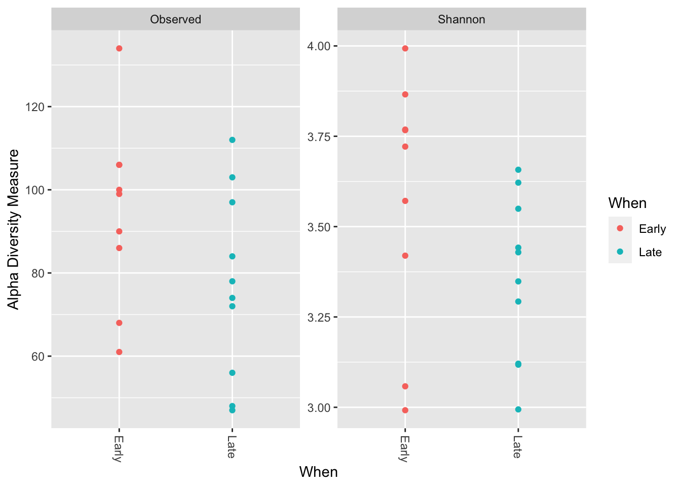
p + labs(x = "", y = "Alpha Diversity Measure\n") +
  theme_bw()
Beta-diversity ordination
ps_rare_bray <- ordinate(ps_rare, "NMDS", "bray")## Square root transformation
## Wisconsin double standardization
## Run 0 stress 0.08484704
## Run 1 stress 0.08484704
## ... New best solution
## ... Procrustes: rmse 2.497137e-06 max resid 5.691675e-06
## ... Similar to previous best
## Run 2 stress 0.09657264
## Run 3 stress 0.08484704
## ... Procrustes: rmse 7.186183e-07 max resid 1.423558e-06
## ... Similar to previous best
## Run 4 stress 0.08484704
## ... Procrustes: rmse 3.303025e-06 max resid 7.565974e-06
## ... Similar to previous best
## Run 5 stress 0.1744901
## Run 6 stress 0.08484704
## ... Procrustes: rmse 1.008148e-06 max resid 2.038791e-06
## ... Similar to previous best
## Run 7 stress 0.08484704
## ... Procrustes: rmse 1.776536e-06 max resid 3.520974e-06
## ... Similar to previous best
## Run 8 stress 0.09657264
## Run 9 stress 0.08484704
## ... Procrustes: rmse 8.550518e-07 max resid 1.794331e-06
## ... Similar to previous best
## Run 10 stress 0.08484704
## ... Procrustes: rmse 1.376679e-06 max resid 2.816876e-06
## ... Similar to previous best
## Run 11 stress 0.08484704
## ... Procrustes: rmse 4.702272e-06 max resid 8.17489e-06
## ... Similar to previous best
## Run 12 stress 0.08484704
## ... New best solution
## ... Procrustes: rmse 2.157179e-07 max resid 4.2813e-07
## ... Similar to previous best
## Run 13 stress 0.08484704
## ... Procrustes: rmse 1.726469e-06 max resid 3.270828e-06
## ... Similar to previous best
## Run 14 stress 0.08484704
## ... Procrustes: rmse 1.055175e-06 max resid 2.649077e-06
## ... Similar to previous best
## Run 15 stress 0.09657265
## Run 16 stress 0.1751066
## Run 17 stress 0.08484704
## ... Procrustes: rmse 6.953774e-07 max resid 1.374792e-06
## ... Similar to previous best
## Run 18 stress 0.09584961
## Run 19 stress 0.08484704
## ... Procrustes: rmse 5.428812e-06 max resid 1.248684e-05
## ... Similar to previous best
## Run 20 stress 0.1795526
## *** Solution reachedplot_ordination(ps_rare, ps_rare_bray, type="samples", color="When") + geom_point(size = 3) 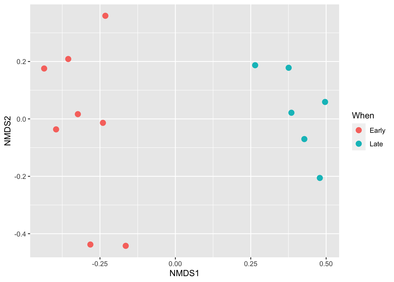
Stacked bar plots
plot_bar(ps, fill="Phylum")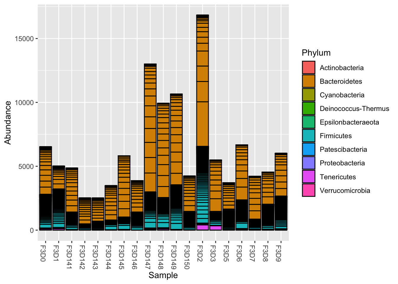
plot_bar(ps_relabund, fill="Phylum") +
  geom_bar(aes(color = Phylum, fill = Phylum), stat="identity", position="stack") +
  labs(x = "", y = "Relative Abundance\n") +
  theme(panel.background = element_blank())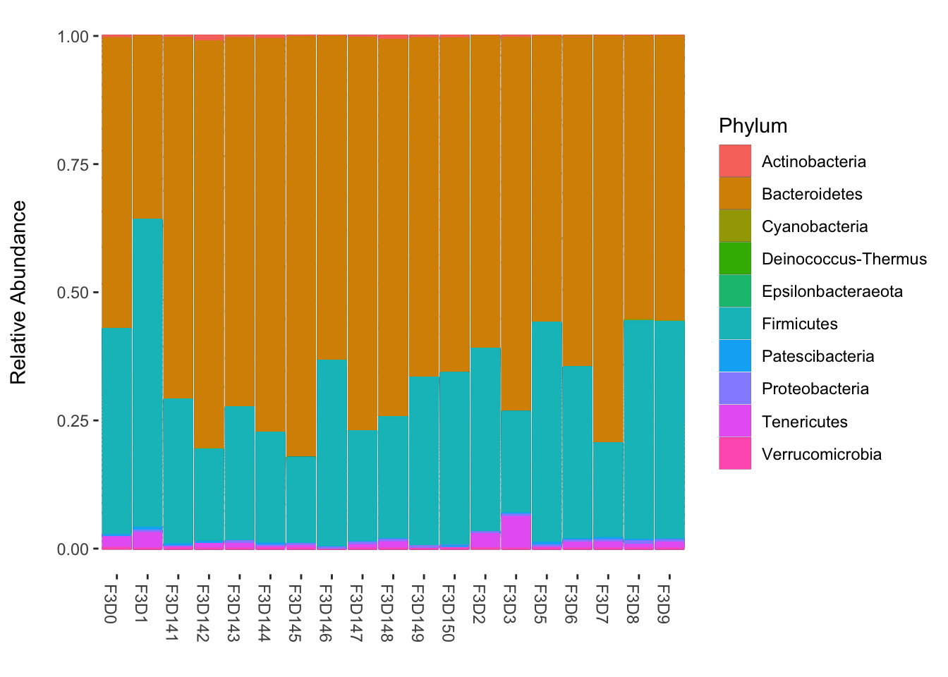
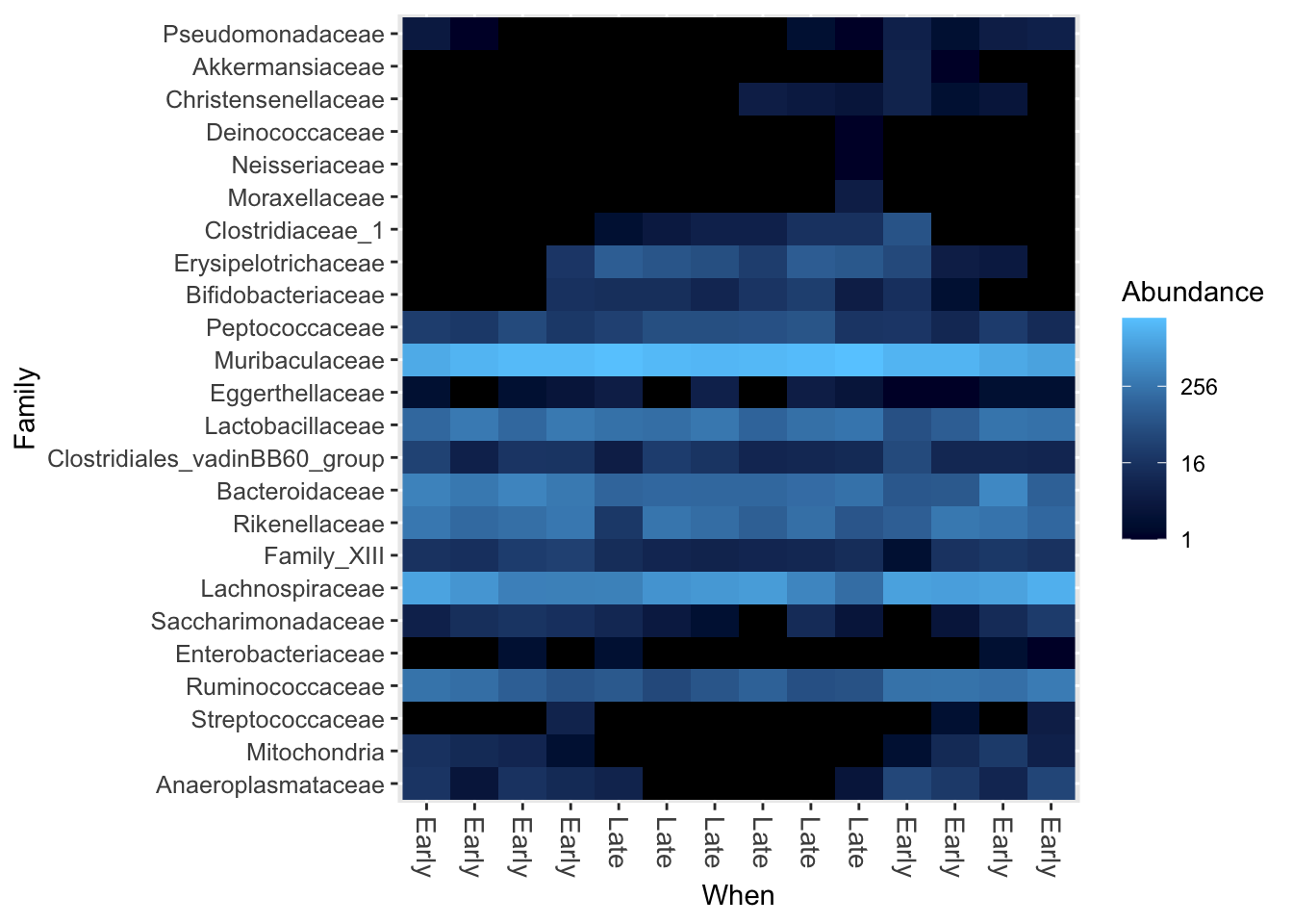
Heatmaps
(ps_fam <- tax_glom(ps, "Family"))## phyloseq-class experiment-level object
## otu_table() OTU Table: [ 33 taxa and 19 samples ]
## sample_data() Sample Data: [ 19 samples by 4 sample variables ]
## tax_table() Taxonomy Table: [ 33 taxa by 7 taxonomic ranks ]
## refseq() DNAStringSet: [ 33 reference sequences ](ps_fam_rare <- rarefy_even_depth(ps_fam, sample.size = 4000, rngseed = 123, replace = FALSE))## `set.seed(123)` was used to initialize repeatable random subsampling.## Please record this for your records so others can reproduce.## Try `set.seed(123); .Random.seed` for the full vector## ...## 5 samples removedbecause they contained fewer reads than `sample.size`.## Up to first five removed samples are:## F3D142F3D143F3D144F3D146F3D5## ...## 9OTUs were removed because they are no longer
## present in any sample after random subsampling## ...## phyloseq-class experiment-level object
## otu_table() OTU Table: [ 24 taxa and 14 samples ]
## sample_data() Sample Data: [ 14 samples by 4 sample variables ]
## tax_table() Taxonomy Table: [ 24 taxa by 7 taxonomic ranks ]
## refseq() DNAStringSet: [ 24 reference sequences ]plot_heatmap(ps_fam_rare, sample.label = "When", taxa.label = "Family")## Warning: Transformation introduced infinite values in discrete y-axis