Sample Size Considerations for Microbiome One-at-a-Time Differential Abundance Testing
I was recently asked how many samples we might need to formally power a differential abundance analysis of prevalent species in the human stool microbiome between “otherwise healthy” control samples and patients with a specific disease condition. Shotgun metagenomic sequencing was going to be employed, the data were to be profiled using MetaPhlAn3, and centered log-ratio regression as implemented by the LinDA method of Zhou et. al. was to be used to identify/screen for differentially abundant species defined as those with a FDR corrected p-value < 0.05.
To do this, we settled on an approach to 1.) simulate data based on a reasonable data generating mechanism for human stool samples profiled via MetaPhlAn3, 2.) fit the linda function to a large number of simulated datasets and extract those meeting the FDR criteria, and 3.) operationalize “average power” as the sensitivity of the test to recover the know differently abundant species (i.e., proportion of positives that are true “spiked” positives).
Fortunately, the Huttenhower lab has developed an excellent tool SparseDOSSA2 that allows one to simulate microbiome data under a zero-inflated log-normal distribution. It can also account for microbial co-occurrence patterns and compositional constraints while allowing users to easily “spike-in” known positive and negative associations to benchmark analysis methods. Their paper, A statistical model for describing and simulating microbial community profiles, describes the method in detail and is available here. We used the human stool template in the package to simulate observed species using parameters obtained from samples collected as part of the Human Microbiome Project. However, the package does include the functionality generate a user-defined templates specific to their environment(s) of interest.
In addition to assessing the sample size required to achieve some level fo average power, we also wanted to assess the expected false positive rate of the LinDA method under the same assumptions since approaches with decent statistical power have generally been found to have inflated FDR rates. Thus, for most microbiome studies employing one-at-a-time differential abundance testing, the proportion of false positives findings is likely in excess of the claimed FDR value…perhaps by a lot.
While I have seen similar numbers presented in other papers, they are always a little eye opening given the current size of most microbiome studies. So, I figured I would share some code in the hopes that it might be helpful to others.
Below I:
- Load the required packages (I am using a slightly dated version of LinDA)
- Assess the sample size required to achieve 80% average power/sensitivity for species seen in at least 30% of samples when 5% of the species are spiked at various log fold changes
- Assess the observed FDR under these same assumptions
- Provide a few thoughts on other simulations that were run, but not included here.
Loading packages
library(tidyverse); packageVersion("tidyverse") ## [1] '1.3.1'library(SparseDOSSA2); packageVersion("SparseDOSSA2") ## [1] '0.99.2'library(phyloseq); packageVersion("phyloseq") ## [1] '1.36.0'library(LinDA); packageVersion("LinDA") ## [1] '0.1.0'library(future.apply); packageVersion("future.apply") ## [1] '1.8.1'Randomly selecting a list of prevalent species to spike
Here I run the SparseDOSSA2 function using the built-in stool template to generate a count matrix comprised of 332 species and 1,000 subjects with a median read depth of 10M reads per sample.
I then retain a list of those species seen in at least 30% of samples that we will be used to randomly spike different species in the subsequent functions.
sim <- SparseDOSSA2(template = "Stool", n_sample = 1000, new_features = FALSE, median_read_depth = 10000000)
sim_df <- data.frame(sim$simulated_data)

prev_sp <- sim_df %>%
  mutate_all(function(x) ifelse(x > 0, 1, 0)) %>%
  mutate_all(as.numeric) %>%
  mutate(Prev = rowMeans(.)) %>%
  rownames_to_column(var = "Species") %>%
  select(Species, Prev) %>%
  filter(Prev >= .3)

rand_sp <- prev_sp$Species

rm(list=ls()[! ls() %in% c("rand_sp")])
Assessing average power
Here I calculate the sensitivity/average power of LinDA to identify the spiked differently abundant species at sample sizes ranging from n=50 to 1,000 and for log fold changes (i.e., effect sizes) of 1, 2, and 4 (log2 fold changes of 0.5, 1, and 2 for those accustomed to the log2 scale).
I also:
- Spike only the relative abundances for 5% of species
- Approximately half are enriched and half depleted in cases (all by the same amount for simplicity)
- An equal number of cases and controls assumed in all simulations (i.e., balanced design)
- Simulate to a median read depth of 10M reads per sample
- Filter taxa at < 30% prevalence (since we usually apply some threshold in our studies)
- Trim/Windsor counts for each species at the 97th percentile to limit the impact of extreme counts on the model estimates
- Drop samples with fewer than 500k reads
- Select an FDR q/p-value of 0.05
As you can see here the nice thing about such a set up is that any of these parameters are modifiable and can be tweaked to your liking or to assess the robustness of results to various settings.
For each combination of sample and effect sizes, I only simulate 100 datasets to speed up this example. For an actual calculation, you would likely want to use a much larger number. I also run the computations in parallel to reduce the run time.
sim_dossa <- function(sample_size, log_fold_up, log_fold_down){
  n_samples <- sample_size

  meta_matrix <- as.matrix(data.frame(
    row.names = paste0(rep("Sample", n_samples), 1:n_samples),
    group = rep(c(0, 1), n_samples / 2)))

  spike_meta_df <- data.frame(
    metadata_datum = rep(1, 17),
    feature_spiked = sample(rand_sp, size = 17, replace = FALSE),
    associated_property = rep("abundance", 17),
    effect_size = c(rep(log_fold_up, 9), rep(log_fold_down, 8)))

  sim <- SparseDOSSA2(template = "Stool", new_features = FALSE, verbose = FALSE,
                      n_sample = sample_size,
                      spike_metadata = spike_meta_df,
                      metadata_matrix = meta_matrix,
                      median_read_depth = 10000000)

  sim_df <- data.frame(sim$simulated_data)

  meta_df <- meta_matrix %>%
    data.frame(.) %>%
    mutate(seq_id = row.names(.))

  ps <- phyloseq(sample_data(meta_df),
                 otu_table(sim_df, taxa_are_rows = TRUE))

  res <- linda(otu.tab = data.frame(otu_table(ps)), meta = data.frame(sample_data(ps)),
               formula = '~ group', alpha = 0.05, winsor.quan = 0.97,
               prev.cut = 0.3, lib.cut = 500000, n.cores = 1)

  res_df <- res$output$group %>%
    rownames_to_column(var = "Species")

  keep_sp <- spike_meta_df$feature_spiked

  tp <- res_df %>%
    filter(Species %in% keep_sp) %>%
    filter(padj < 0.05)

  fn <- res_df %>%
    filter(Species %in% keep_sp) %>%
    filter(padj > 0.05)

  power <- nrow(tp) / (nrow(tp) + nrow(fn))

  return(power)
}

plan(multisession, gc = TRUE, workers = 6)

sim_power_df <- data.frame(
  n = rep(c(50, 100, 200, 400, 600, 800, 1000), each = 3),
  log_fold = rep(c(1, 2, 4), 7),
  power = c(
    lf1_n50 = round(mean(future_replicate(100, sim_dossa(sample_size = 50, log_fold_up = 1, log_fold_down = -1))), 2),
    lf2_n50 = round(mean(future_replicate(100, sim_dossa(sample_size = 50, log_fold_up = 2, log_fold_down = -2))), 2),
    lf3_n50 = round(mean(future_replicate(100, sim_dossa(sample_size = 50, log_fold_up = 4, log_fold_down = -4))), 2),

    lf1_n100 = round(mean(future_replicate(100, sim_dossa(sample_size = 100, log_fold_up = 1, log_fold_down = -1))), 2),
    lf2_n100 = round(mean(future_replicate(100, sim_dossa(sample_size = 100, log_fold_up = 2, log_fold_down = -2))), 2),
    lf3_n100 = round(mean(future_replicate(100, sim_dossa(sample_size = 100, log_fold_up = 4, log_fold_down = -4))), 2),

    lf1_n200 = round(mean(future_replicate(100, sim_dossa(sample_size = 200, log_fold_up = 1, log_fold_down = -1))), 2),
    lf2_n200 = round(mean(future_replicate(100, sim_dossa(sample_size = 200, log_fold_up = 2, log_fold_down = -2))), 2),
    lf3_n200 = round(mean(future_replicate(100, sim_dossa(sample_size = 200, log_fold_up = 4, log_fold_down = -4))), 2),

    lf1_n400 = round(mean(future_replicate(100, sim_dossa(sample_size = 400, log_fold_up = 1, log_fold_down = -1))), 2),
    lf2_n400 = round(mean(future_replicate(100, sim_dossa(sample_size = 400, log_fold_up = 2, log_fold_down = -2))), 2),
    lf3_n400 = round(mean(future_replicate(100, sim_dossa(sample_size = 400, log_fold_up = 4, log_fold_down = -4))), 2),

    lf1_n600 = round(mean(future_replicate(100, sim_dossa(sample_size = 600, log_fold_up = 1, log_fold_down = -1))), 2),
    lf2_n600 = round(mean(future_replicate(100, sim_dossa(sample_size = 600, log_fold_up = 2, log_fold_down = -2))), 2),
    lf3_n600 = round(mean(future_replicate(100, sim_dossa(sample_size = 600, log_fold_up = 4, log_fold_down = -4))), 2),

    lf1_n800 = round(mean(future_replicate(100, sim_dossa(sample_size = 800, log_fold_up = 1, log_fold_down = -1))), 2),
    lf2_n800 = round(mean(future_replicate(100, sim_dossa(sample_size = 800, log_fold_up = 2, log_fold_down = -2))), 2),
    lf3_n800 = round(mean(future_replicate(100, sim_dossa(sample_size = 800, log_fold_up = 4, log_fold_down = -4))), 2),

    lf1_n1000 = round(mean(future_replicate(100, sim_dossa(sample_size = 1000, log_fold_up = 1, log_fold_down = -1))), 2),
    lf2_n1000 = round(mean(future_replicate(100, sim_dossa(sample_size = 1000, log_fold_up = 2, log_fold_down = -2))), 2),
    lf3_n1000 = round(mean(future_replicate(100, sim_dossa(sample_size = 1000, log_fold_up = 4, log_fold_down = -4))), 2)
  )
)
ggplot(data = sim_power_df, aes(x = n, y = power, group = as.factor(log_fold), color = as.factor(log_fold))) +
geom_point() +
geom_line() +
scale_x_continuous(breaks=seq(50, 1000, 100)) +
labs(x = "\nSample Size", y = "Sensitivity\n", color = "Log Fold Change") +
theme(legend.position = "bottom")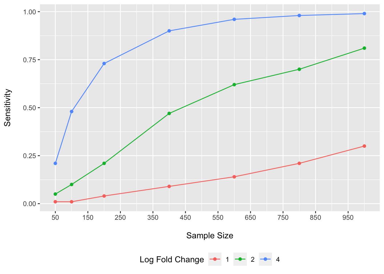
As we can see, very large sample sizes would be required to reliably detect log fold changes of 1.
To achieve 80% sensitivity for a log fold change of 2 (log2 = 1), we would need somewhere around n=1000 participant samples under this scenario.
To achieve 80% sensitivity for a log fold change of 4 (log2 = 2), we would need somewhere around n=300 participant samples.
Plausible values for expected fold changes would be expected to differ for various comparisons/experimental conditions. However, another issue we face is that when we get into log fold changes of 4 for 5% of species, we are starting to posit some somewhat large effect sizes for a fair number of species. The ability of current methods to account for the compositional bias in this setting may be expected to start to break down. So lets look at that now.
Assessing control of the FDR
Here we examine the distribution of the empirical FDR under the same assumptions as provided above for power/sensitivity.
sim_dossa_fdr <- function(sample_size, log_fold_up, log_fold_down){
  n_samples <- sample_size

  meta_matrix <- as.matrix(data.frame(
    row.names = paste0(rep("Sample", n_samples), 1:n_samples),
    group = rep(c(0, 1), n_samples / 2)))

  spike_meta_df <- data.frame(
    metadata_datum = rep(1, 17),
    feature_spiked = sample(rand_sp, size = 17, replace = FALSE),
    associated_property = rep("abundance", 17),
    effect_size = c(rep(log_fold_up, 9), rep(log_fold_down, 8)))

  sim <- SparseDOSSA2(template = "Stool", new_features = FALSE, verbose = FALSE,
                      n_sample = sample_size,
                      spike_metadata = spike_meta_df,
                      metadata_matrix = meta_matrix,
                      median_read_depth = 10000000)

  sim_df <- data.frame(sim$simulated_data)

  meta_df <- meta_matrix %>%
    data.frame(.) %>%
    mutate(seq_id = row.names(.))

  ps <- phyloseq(sample_data(meta_df),
                 otu_table(sim_df, taxa_are_rows = TRUE))

  res <- linda(otu.tab = data.frame(otu_table(ps)), meta = data.frame(sample_data(ps)),
               formula = '~ group', alpha = 0.05, winsor.quan = 0.97,
               prev.cut = 0.3, lib.cut = 500000, n.cores = 1)

  res_df <- res$output$group %>%
    rownames_to_column(var = "Species")

  keep_sp <- spike_meta_df$feature_spiked

  tp <- res_df %>%
    filter(Species %in% keep_sp) %>%
    filter(padj < 0.05)

  fp <- res_df %>%
    filter(!(Species %in% keep_sp)) %>%
    filter(padj < 0.05)

  fdr <- nrow(fp) / (nrow(fp) + nrow(tp))

  fdr <- ifelse(is.nan(fdr), 0, fdr)

  return(fdr)
}

plan(multisession, gc = TRUE, workers = 6)

lf1_n50 <- data.frame(n = 50, log_fold = 1, fdr = future_replicate(100, sim_dossa_fdr(sample_size = 50, log_fold_up = 1, log_fold_down = -1)))
lf2_n50 <- data.frame(n = 50, log_fold = 2, fdr = future_replicate(100, sim_dossa_fdr(sample_size = 50, log_fold_up = 2, log_fold_down = -2)))
lf3_n50 <- data.frame(n = 50, log_fold = 4, fdr = future_replicate(100, sim_dossa_fdr(sample_size = 50, log_fold_up = 4, log_fold_down = -4)))

lf1_n100 <- data.frame(n = 100, log_fold = 1, fdr = future_replicate(100, sim_dossa_fdr(sample_size = 100, log_fold_up = 1, log_fold_down = -1)))
lf2_n100 <- data.frame(n = 100, log_fold = 2, fdr = future_replicate(100, sim_dossa_fdr(sample_size = 100, log_fold_up = 2, log_fold_down = -2)))
lf3_n100 <- data.frame(n = 100, log_fold = 4, fdr = future_replicate(100, sim_dossa_fdr(sample_size = 100, log_fold_up = 4, log_fold_down = -4)))

lf1_n200 <- data.frame(n = 200, log_fold = 1, fdr = future_replicate(100, sim_dossa_fdr(sample_size = 200, log_fold_up = 1, log_fold_down = -1)))
lf2_n200 <- data.frame(n = 200, log_fold = 2, fdr = future_replicate(100, sim_dossa_fdr(sample_size = 200, log_fold_up = 2, log_fold_down = -2)))
lf3_n200 <- data.frame(n = 200, log_fold = 4, fdr = future_replicate(100, sim_dossa_fdr(sample_size = 200, log_fold_up = 4, log_fold_down = -4)))

lf1_n400 <- data.frame(n = 400, log_fold = 1, fdr = future_replicate(100, sim_dossa_fdr(sample_size = 400, log_fold_up = 1, log_fold_down = -1)))
lf2_n400 <- data.frame(n = 400, log_fold = 2, fdr = future_replicate(100, sim_dossa_fdr(sample_size = 400, log_fold_up = 2, log_fold_down = -2)))
lf3_n400 <- data.frame(n = 400, log_fold = 4, fdr = future_replicate(100, sim_dossa_fdr(sample_size = 400, log_fold_up = 4, log_fold_down = -4)))

lf1_n600 <- data.frame(n = 600, log_fold = 1, fdr = future_replicate(100, sim_dossa_fdr(sample_size = 600, log_fold_up = 1, log_fold_down = -1)))
lf2_n600 <- data.frame(n = 600, log_fold = 2, fdr = future_replicate(100, sim_dossa_fdr(sample_size = 600, log_fold_up = 2, log_fold_down = -2)))
lf3_n600 <- data.frame(n = 600, log_fold = 4, fdr = future_replicate(100, sim_dossa_fdr(sample_size = 600, log_fold_up = 4, log_fold_down = -4)))

lf1_n800 <- data.frame(n = 800, log_fold = 1, fdr = future_replicate(100, sim_dossa_fdr(sample_size = 800, log_fold_up = 1, log_fold_down = -1)))
lf2_n800 <- data.frame(n = 800, log_fold = 2, fdr = future_replicate(100, sim_dossa_fdr(sample_size = 800, log_fold_up = 2, log_fold_down = -2)))
lf3_n800 <- data.frame(n = 800, log_fold = 4, fdr = future_replicate(100, sim_dossa_fdr(sample_size = 800, log_fold_up = 4, log_fold_down = -4)))

lf1_n1000 <- data.frame(n = 1000, log_fold = 1, fdr = future_replicate(100, sim_dossa_fdr(sample_size = 1000, log_fold_up = 1, log_fold_down = -1)))
lf2_n1000 <- data.frame(n = 1000, log_fold = 2, fdr = future_replicate(100, sim_dossa_fdr(sample_size = 1000, log_fold_up = 2, log_fold_down = -2)))
lf3_n1000 <- data.frame(n = 1000, log_fold = 4, fdr = future_replicate(100, sim_dossa_fdr(sample_size = 1000, log_fold_up = 4, log_fold_down = -4)))

sim_fdr_df <- bind_rows(lf1_n50, lf2_n50, lf3_n50, lf1_n100, lf2_n100, lf3_n100,
                        lf1_n200, lf2_n200, lf3_n200, lf1_n400, lf2_n400, lf3_n400,
                        lf1_n600, lf2_n600, lf3_n600, lf1_n800, lf2_n800, lf3_n800,
                        lf1_n1000, lf2_n1000, lf3_n1000)
ggplot(data = sim_fdr_df, aes(x = as.factor(log_fold), y = fdr)) +
geom_boxplot(outlier.shape = NA) +
geom_jitter(height = 0, width = 0.2, aes(color = as.factor(log_fold))) +
stat_summary(fun.y="mean", shape = 18) +
geom_hline(yintercept = 0.05, linetype = "dashed", color = "red") +
labs(x = "\nLog Fold Change", y = "FDR\n") +
facet_wrap(~n) +
theme(legend.position = "none")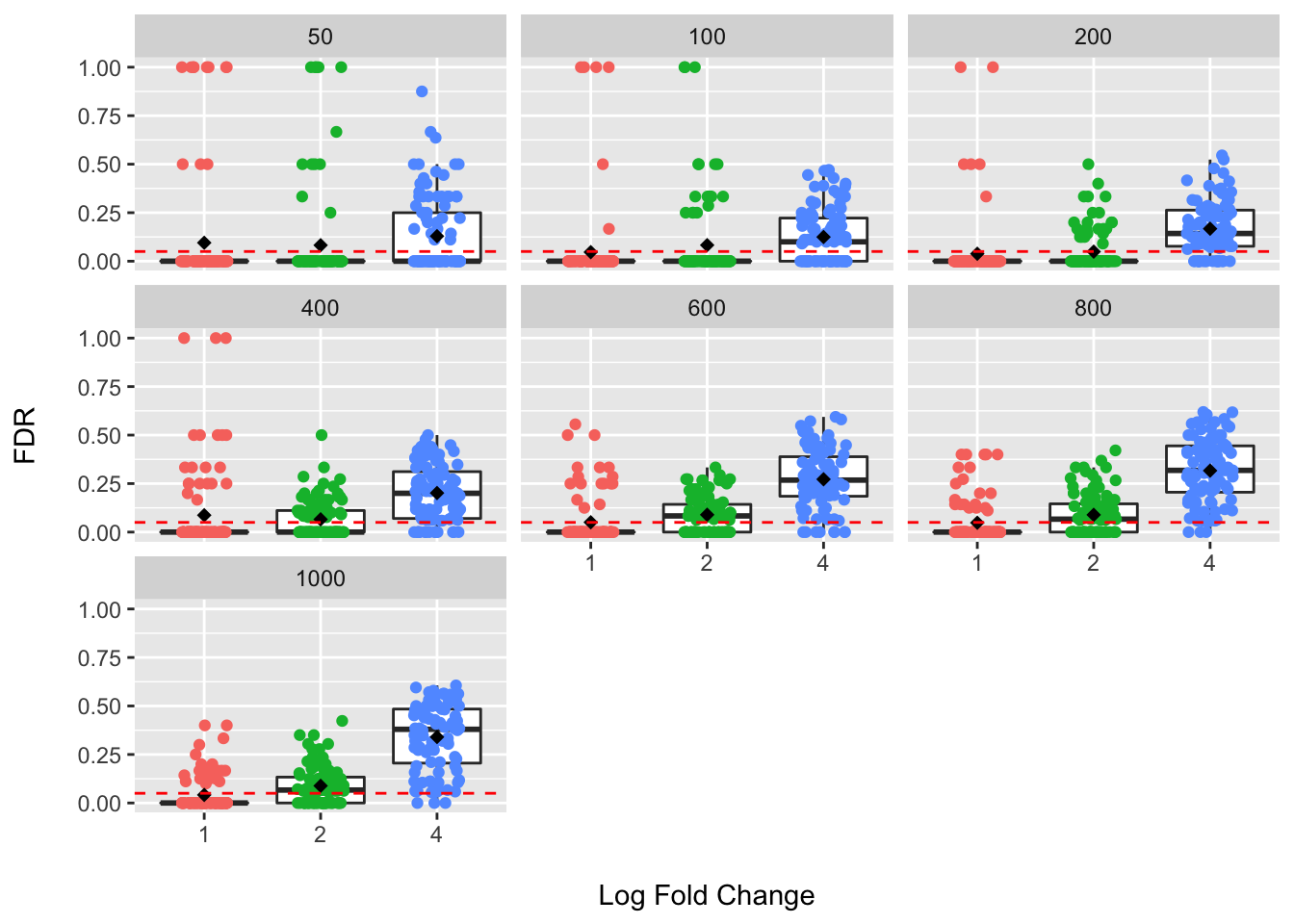
Here the red dashed line provides the claimed FDR value of 5%. The line of the box plot provides the median, and the star the mean, value over 100 simulated datasets for each sample and effect size combination. What we hope to see is that the observed FDR values do not exceed the claimed value.
For log fold changes of 1 and 2, we can see that the mean and median values look to be near the claimed FDR value; however, we do see a fair number of datasets where the claimed value was exceeded…sometimes by a lot!
At a log fold change of 4, we can see that the claimed FDR threshold is largely exceeded under these assumptions and larger sample sizes to not help address this problem. This means that many more false positive species are being flagged as differentially abundant than we think based on our chosen FDR level. Assuming our simulation has some basis in reality, this is a major concern for these types of methods (among others) and would be expected to contribute to poor reproducibility and to chasing down leads in experimental settings that are false positive results. See the MaAsLin2 paper where they used a similar approach examining the sensitivity and FDR for a large number of models and found that, similar to many others, that most methods exhibited an inflated average FDR.
Other simuation results not shown
I ran a much more extensive set of simulations than shown here. Some things I observed were that:
- LinDA did as well or better than the default approach in MaAsLin2 over a range of parameters. Thus, based on this simulation set up, it did as well (or better) as the best previously performing model (based on sparseDossa simulated data).
- DESeq2 was found to provide improvements in sensitivity/average power…although it generally came at the cost of worse FDR control (as others have reported). So perhaps a reasonable choice for small samples, but beware of false positives.
- Zero-inflated negative binomial regression focused on the abundance parameter had poor FDR control as reported in the MaAsLin2 paper.
Take away
All-in-all, it seems that if one is to pursue one-at-time feature testing that samples sizes much larger than are commonly reported for microbiome studies are needed to reliably detect differences for more moderate effect sizes. In addition, replication/validation of features flagged as differentially abundant is critically important given current limitations in controlling the FDR.
sessionInfo()## R version 4.1.1 (2021-08-10)
## Platform: x86_64-apple-darwin17.0 (64-bit)
## Running under: macOS Catalina 10.15.7
##
## Matrix products: default
## BLAS: /Library/Frameworks/R.framework/Versions/4.1/Resources/lib/libRblas.0.dylib
## LAPACK: /Library/Frameworks/R.framework/Versions/4.1/Resources/lib/libRlapack.dylib
##
## locale:
## [1] en_US.UTF-8/en_US.UTF-8/en_US.UTF-8/C/en_US.UTF-8/en_US.UTF-8
##
## attached base packages:
## [1] stats graphics grDevices utils datasets methods base
##
## other attached packages:
## [1] LinDA_0.1.0 phyloseq_1.36.0 SparseDOSSA2_0.99.2
## [4] Rmpfr_0.8-7 gmp_0.6-2 igraph_1.2.7
## [7] truncnorm_1.0-8 magrittr_2.0.1 future.apply_1.8.1
## [10] future_1.22.1 huge_1.3.5 mvtnorm_1.1-3
## [13] ks_1.13.3 forcats_0.5.1 stringr_1.4.0
## [16] dplyr_1.0.7 purrr_0.3.4 readr_2.0.2
## [19] tidyr_1.1.4 tibble_3.1.5 ggplot2_3.3.5
## [22] tidyverse_1.3.1
##
## loaded via a namespace (and not attached):
## [1] readxl_1.3.1 backports_1.2.1 plyr_1.8.6
## [4] splines_4.1.1 listenv_0.8.0 GenomeInfoDb_1.28.4
## [7] digest_0.6.28 foreach_1.5.1 htmltools_0.5.2
## [10] lmerTest_3.1-3 fansi_0.5.0 cluster_2.1.2
## [13] tzdb_0.1.2 globals_0.14.0 Biostrings_2.60.2
## [16] modelr_0.1.8 stabledist_0.7-1 colorspace_2.0-2
## [19] rvest_1.0.2 ggrepel_0.9.1 haven_2.4.3
## [22] xfun_0.29 crayon_1.4.1 RCurl_1.98-1.5
## [25] jsonlite_1.7.2 lme4_1.1-27.1 survival_3.2-11
## [28] iterators_1.0.13 ape_5.5 glue_1.4.2
## [31] gtable_0.3.0 zlibbioc_1.38.0 XVector_0.32.0
## [34] Rhdf5lib_1.14.2 BiocGenerics_0.38.0 scales_1.1.1
## [37] DBI_1.1.1 Rcpp_1.0.7 clue_0.3-60
## [40] mclust_5.4.7 stats4_4.1.1 timeSeries_3062.100
## [43] httr_1.4.2 ellipsis_0.3.2 spatial_7.3-14
## [46] farver_2.1.0 pkgconfig_2.0.3 sass_0.4.0
## [49] dbplyr_2.1.1 utf8_1.2.2 labeling_0.4.2
## [52] tidyselect_1.1.1 rlang_0.4.12 reshape2_1.4.4
## [55] munsell_0.5.0 cellranger_1.1.0 tools_4.1.1
## [58] cli_3.1.0 generics_0.1.1 ade4_1.7-18
## [61] broom_0.7.9 evaluate_0.14 biomformat_1.20.0
## [64] fastmap_1.1.0 yaml_2.2.1 knitr_1.36
## [67] fs_1.5.0 nlme_3.1-152 pracma_2.3.3
## [70] xml2_1.3.2 compiler_4.1.1 rstudioapi_0.13
## [73] reprex_2.0.1 bslib_0.3.1 stringi_1.7.5
## [76] statip_0.2.3 highr_0.9 blogdown_1.7
## [79] modeest_2.4.0 lattice_0.20-44 fBasics_3042.89.1
## [82] Matrix_1.3-4 nloptr_1.2.2.2 vegan_2.5-7
## [85] permute_0.9-5 multtest_2.48.0 vctrs_0.3.8
## [88] pillar_1.6.4 lifecycle_1.0.1 rhdf5filters_1.4.0
## [91] jquerylib_0.1.4 data.table_1.14.2 bitops_1.0-7
## [94] R6_2.5.1 stable_1.1.4 bookdown_0.24
## [97] KernSmooth_2.23-20 IRanges_2.26.0 parallelly_1.28.1
## [100] codetools_0.2-18 boot_1.3-28 MASS_7.3-54
## [103] assertthat_0.2.1 rhdf5_2.36.0 withr_2.4.2
## [106] S4Vectors_0.30.2 GenomeInfoDbData_1.2.6 mgcv_1.8-36
## [109] parallel_4.1.1 hms_1.1.1 grid_4.1.1
## [112] rpart_4.1-15 timeDate_3043.102 minqa_1.2.4
## [115] rmarkdown_2.11 rmutil_1.1.5 numDeriv_2016.8-1.1
## [118] Biobase_2.52.0 lubridate_1.8.0