Sample Size Considerations for Microbial Metagenomics Research
One of the most common questions we get from investigators at the Microbial Metagenomics Analysis Center (MMAC) is how many samples should I collect for my study? Even once we have a clearly stated and testable hypothesis, this is not always easy, since sample size calculations for microbiome studies are typically not amenable to closed form solutions (i.e., plug-in formulas) and require us to make, sometimes complex, assumptions about the underlying data generating process (DGP).
An important observation made as part of the first Human Microbiome Project was the large degree of inter-individual variation in the human microbiome leading to high-dimensional and sparse taxonomic and functional/gene profiles. Given most species (or strains, gene families, etc.) would not be expected to be present in some proportion of participants, but may have a large relative abundance in others, we need a DGP that reflects this assumption. There are several ways to go about this, but mixture distributions are one option where the data are simulated as two parts: 1.) the probability of observance and 2.) drawing values from some probability distribution for those participants in whom the probability of observance is non-zero. So, if we are willing to make some (hopefully reasonable) assumptions, and we have a test of interest, we can obtain estimates of statistical power using a simulation-based approach where we draw many samples of a given sample size and then determine whether or not the results meet some criteria (often a p-value < 0.05). The proportion of times the criteria is met provides us with an empirical estimate of study power. Easy enough in principle, hard in practice.
Below I provide a few examples of how we might consider approaching sample size calculations based on hypotheses about single species in the MMAC. I focus mainly on sample size calculations for testing for differences in the relative abundance of a single taxa since, at current, I am of the opinion that well-articulated questions based on a priori assumed mechanisms of action are preferable whenever possible. Aggregating species or genes in some principled way prior to testing is likely an improvement in many cases over testing single species or genes (i.e., assumption that species or genes operate in isolation likely not often best one we could make), but beyond the scope of the examples provided here. I also show some examples of how one might power on measures of alpha- and beta-diversity should those be of interest. See my previous post Sample Size Considerations for Microbiome One-at-a-Time Differential Abundance Testing if you are interested in how you might approach a sample size determination for differential abundance testing of a large number of different species.
I always recommend running a small pilot first if at all possible. This serves several purposes. First, estimates for many of the parameters we will need are hard to guess at. So best to have pilot data on the exact study population(s) of interest from which to obtain quantitative estimates for these parameters. Second, if we have a decent sized pilot study, we can resample from that dataset to obtain estimates of statistical power for larger sample sizes. The assumptions required to obtain accurate estimates via resampling might not always be met exactly in practice, but may be better than the assumptions for the DGP we make when generating the simulations (i.e., the pilot may reflect features of the data we miss in our simulation). The downside is that it is a bit tricker to modify aspects of the data (i.e, effect size) with resampling. If you are not able to run a pilot, then given the amount of publicly available microbiome data, reach out to us and we can likely find something to serve as a reasonable template for the calculations. Third, it will give you an opportunity to work through the various practical difficulties of running the study and to what identify what other difficulties might arise (i.e., lower than expected return to biospecimens, etc.).
I only show examples for a two-group balanced design here, but these approaches can be modified to reflect other study designs (i.e., continuous exposures, multiple groups, repeated measures, etc.).
Load libraries
library(tidyverse); packageVersion("tidyverse")## [1] '1.3.1'library(curatedMetagenomicData); packageVersion("curatedMetagenomicData")## [1] '3.0.10'library(phyloseq); packageVersion("phyloseq")## [1] '1.36.0'library(microbiome); packageVersion("microbiome")## [1] '1.14.0'library(pscl); packageVersion("pscl")## [1] '1.5.5'library(future.apply); packageVersion("future.apply") ## [1] '1.8.1'library(cowplot); packageVersion("cowplot")## [1] '1.1.1'library(broom); packageVersion("broom")## [1] '0.7.9'library(pwr); packageVersion("pwr")## [1] '1.3.0'library(vegan); packageVersion("vegan")## [1] '2.5.7'library(Hmisc); packageVersion("Hmisc")## [1] '4.6.0'library(SparseDOSSA2); packageVersion("SparseDOSSA2")## [1] '0.99.2'Grab some example pilot data
In this code chunk, I pull down some data from the The Integrative Human Microbiome Project IBD project available via the curatedMetagenomicData package to serve as “example” pilot data.
These are stool samples collected from participants with IBD and healthy controls. I retain all the distinct baseline samples from the healthy controls and randomly select 20 from those with IBD to better approximate the size of a pilot study.
I then convert the data into a phyloseq object and print/plot some of the data elements to get a feel for the characteristics of participants providing samples.
meta_df <- curatedMetagenomicData::sampleMetadata

mydata <- meta_df %>%
  dplyr::filter(study_name == "HMP_2019_ibdmdb") %>%
  dplyr::filter(visit_number == 1) %>%
  dplyr::select(study_name, sample_id, subject_id, body_site, disease, age, gender, BMI, country, visit_number) %>%
  na.omit(.) %>%
  distinct(subject_id, .keep_all = TRUE)

ibd_df <- mydata %>%
  filter(disease == "IBD")

set.seed(234)
keep_ids <- sample(ibd_df$subject_id, size = 20, replace = FALSE)

mydata <- mydata %>%
  filter(disease == "healthy" | subject_id %in% keep_ids)

keep_id <- mydata$sample_id

crc_se_sp <- sampleMetadata %>%
  dplyr::filter(sample_id %in% keep_id) %>%
  curatedMetagenomicData::returnSamples("relative_abundance", counts = TRUE)

crc_sp_df <- as.data.frame(as.matrix(assay(crc_se_sp)))

crc_sp_df <- crc_sp_df %>%
  rownames_to_column(var = "Species")

otu_tab <- crc_sp_df %>%
  tidyr::separate(Species, into = c("Kingdom", "Phylum", "Class", "Order", "Family", "Genus", "Species"), sep = "\\|") %>%
  dplyr::select(-Kingdom, -Phylum, -Class, -Order, -Family, -Genus) %>%
  dplyr::mutate(Species = gsub("s__", "", Species)) %>%
  tibble::column_to_rownames(var = "Species")

tax_tab <- crc_sp_df %>%
  dplyr::select(Species) %>%
  tidyr::separate(Species, into = c("Kingdom", "Phylum", "Class", "Order", "Family", "Genus", "Species"), sep = "\\|") %>%
  dplyr::mutate(Kingdom = gsub("k__", "", Kingdom),
                Phylum = gsub("p__", "", Phylum),
                Class = gsub("c__", "", Class),
                Order = gsub("o__", "", Order),
                Family = gsub("f__", "", Family),
                Genus = gsub("g__", "", Genus),
                Species = gsub("s__", "", Species)) %>%
  dplyr::mutate(spec_row = Species) %>%
  tibble::column_to_rownames(var = "spec_row")

meta_df <- mydata %>%
  tibble::column_to_rownames(var = "sample_id")

(ps <- phyloseq(sample_data(meta_df),
                otu_table(otu_tab, taxa_are_rows = TRUE),
                tax_table(as.matrix(tax_tab))))

rm(list=setdiff(ls(), "ps"))
sample_data(ps) %>%
data.frame() %>%
dplyr::select(-age, -BMI) %>%
Hmisc::describe(.)## .
##
## 7 Variables 40 Observations
## --------------------------------------------------------------------------------
## study_name
## n missing distinct value
## 40 0 1 HMP_2019_ibdmdb
##
## Value HMP_2019_ibdmdb
## Frequency 40
## Proportion 1
## --------------------------------------------------------------------------------
## subject_id
## n missing distinct
## 40 0 40
##
## lowest : C3005 C3010 C3034 C3035 E5004, highest: P6012 P6014 P6018 P6024 P6025
## --------------------------------------------------------------------------------
## body_site
## n missing distinct value
## 40 0 1 stool
##
## Value stool
## Frequency 40
## Proportion 1
## --------------------------------------------------------------------------------
## disease
## n missing distinct
## 40 0 2
##
## Value healthy IBD
## Frequency 20 20
## Proportion 0.5 0.5
## --------------------------------------------------------------------------------
## gender
## n missing distinct
## 40 0 2
##
## Value female male
## Frequency 19 21
## Proportion 0.475 0.525
## --------------------------------------------------------------------------------
## country
## n missing distinct value
## 40 0 1 USA
##
## Value USA
## Frequency 40
## Proportion 1
## --------------------------------------------------------------------------------
## visit_number
## n missing distinct Info Mean Gmd
## 40 0 1 0 1 0
##
## Value 1
## Frequency 40
## Proportion 1
## --------------------------------------------------------------------------------sample_data(ps) %>%
data.frame() %>%
dplyr::select(age, BMI, disease) %>%
pivot_longer(!disease, names_to = "group", values_to = "value") %>%
ggplot((aes(x = disease, y = value, color = disease))) +
geom_point() +
labs(x = "", y = "") +
facet_wrap(~group, scales = "free_y") +
theme(legend.position = "none")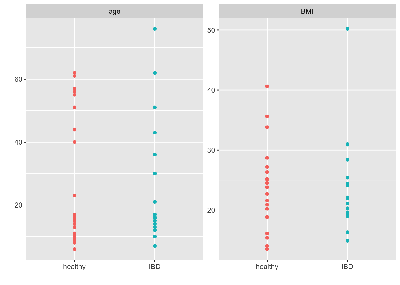
All-in-all this looks pretty good (i.e., I grabbed what looks to be the right samples and we have some balance in terms of gender, age, BMI etc.). This will suffice for our purposes.
Simulate observed E.coli distribution
For these examples, I will assume we are interested in better understanding how many samples we might require to power a test of differential abundance in E.coli between healthy controls and patients with IBD. I have no real interest in the role E.coli in IBD per se, I just selected this species since I expect everyone has some familiarity.
First, I plot the observed distribution of reads classified to E.coli via MetaPhlAn3.
ps_ecoli <- subset_taxa(ps, Species == "Escherichia_coli")
ecoli_df <- data.frame(t((otu_table(ps_ecoli))))

(p1 <- ggplot(ecoli_df, aes(x = Escherichia_coli)) +
    geom_histogram(aes(y = ..density..), colour = 1, fill = "white", bins = 60) +
    geom_density(lwd = 1.2, linetype = 2, colour = 2) +
    labs(x = "\nE.coli Read Counts", y = "Density\n") +
    ggtitle("Observed"))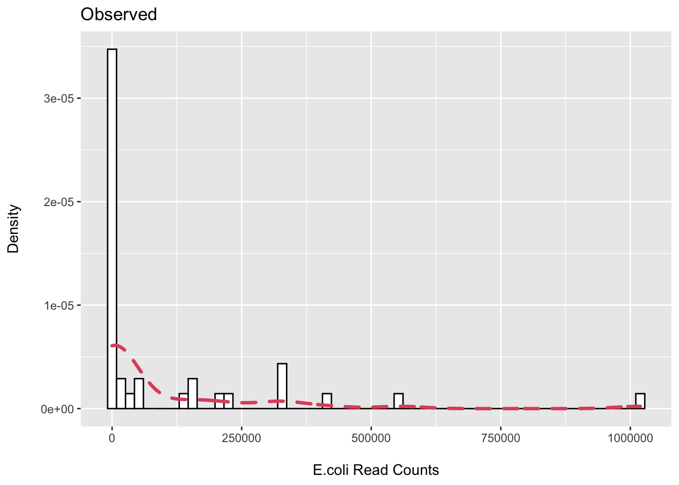
ecoli_df %>%
  filter(Escherichia_coli == 0) %>%
  summarise(n = n())
## n
## 1 19We can see that we have about ~50% zeros then wide distribution of samples with observed counts.
Let’s see if we can get close to approximating this using a zero-inflated negative binomial (ZINB) distribution. This is a mixture distribution where the probability of being a zero (structural) is modeled by a binomial distribution and the non-zero values by the negative binomial. Here is an example of fitting the ZINB in R.
m <- zeroinfl(Escherichia_coli ~ 1, data = ecoli_df, dist = "negbin")
summary(m)
##
## Call:
## zeroinfl(formula = Escherichia_coli ~ 1, data = ecoli_df, dist = "negbin")
##
## Pearson residuals:
## Min 1Q Median 3Q Max
## -0.4787 -0.4787 -0.4639 0.1924 4.3582
##
## Count model coefficients (negbin with log link):
## Estimate Std. Error z value Pr(>|z|)
## (Intercept) 12.1649 0.2942 41.344 <2e-16 ***
## Log(theta) -0.5981 0.2641 -2.265 0.0235 *
##
## Zero-inflation model coefficients (binomial with logit link):
## Estimate Std. Error z value Pr(>|z|)
## (Intercept) -0.102 0.317 -0.322 0.748
## ---
## Signif. codes: 0 '***' 0.001 '**' 0.01 '*' 0.05 '.' 0.1 ' ' 1
##
## Theta = 0.5498
## Number of iterations in BFGS optimization: 5
## Log-likelihood: -301 on 3 Dfn <- 40
zero_prob <- .50
set.seed(243)
z <- rbinom(n = n, size = 1, prob = 1 - zero_prob)
y <- ifelse(z == 0, 0,
rnbinom(n = n,
mu = exp(12.2),
size = .55))
sim_ecoli <- data.frame(Escherichia_coli = y)
p2 <- ggplot(sim_ecoli, aes(x = Escherichia_coli)) +
geom_histogram(aes(y = ..density..), colour = 1, fill = "white", bins = 60) +
geom_density(lwd = 1.2, linetype = 2, colour = 2) +
labs(x = "\nE.coli Read Counts", y = "Density\n") +
ggtitle("Simulated")
cowplot::plot_grid(p1, p2, scale = .9)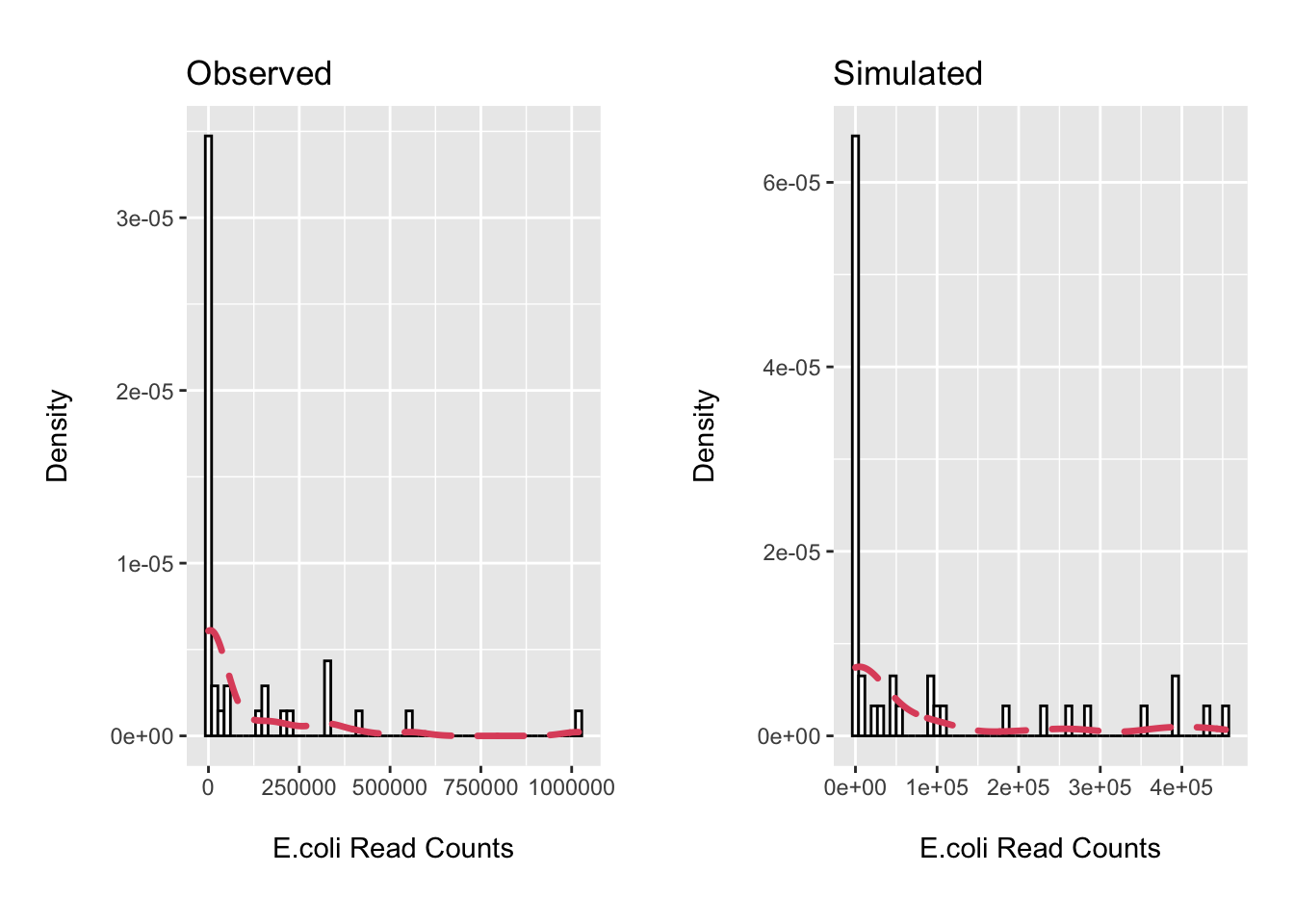
rm(list=setdiff(ls(), c("ps", "ecoli_df")))Not terrible. We will use the ZINB mixture distribution for our simulations.
Assess effect size in pilot data
Here we will fit the ZINB model to the pilot data to get the observed effect size and the estimates for the intercept, log mean difference, and variance/theta parameters we will need to write the two group simulation. Typically one would then make assumptions about the minimum detectable effect size of interest for which to power on when performing the sample size determination. However, in this example, I will use the observed effect size to see how well it corresponds to the resampling-based approach.
Also, I do not explicitly account for differences in library depth between samples in these examples. I would not expect it to make too much difference here, but this could be done by including a scaling factor as a model offset (on the log scale) that reflects the differences in the library sizes. See my previous post where I show how one could use wrench or GMPR to obtain such scaling factors.
I also focus on the count distribution of the model (i.e., assume our interest is for those in which we expect the probability of observing the species is non-zero). One could integrate the estimates for the zero and count components if that is of interest. See the chapter “Modeling Zero-Inflated Microbiome Data” in Xia, Sun, and Chen’s textbook Statistical Analysis of Microbiome Data with R for an example.
ecoli_df <- ecoli_df %>%
  rownames_to_column(var = "seq_id")

meta_df <- data.frame(sample_data(ps)) %>%
  rownames_to_column(var = "seq_id") %>%
  dplyr::select(seq_id, disease)

ecoli_df <- left_join(ecoli_df, meta_df)

ecoli_df <- ecoli_df %>%
  mutate(disease = factor(disease, levels = c("healthy", "IBD")))

m_pilot <- zeroinfl(Escherichia_coli ~ disease | 1, data = ecoli_df, dist = "negbin")
summary(m_pilot)
##
## Call:
## zeroinfl(formula = Escherichia_coli ~ disease | 1, data = ecoli_df, dist = "negbin")
##
## Pearson residuals:
## Min 1Q Median 3Q Max
## -0.490082 -0.490082 -0.473742 -0.008637 2.948623
##
## Count model coefficients (negbin with log link):
## Estimate Std. Error z value Pr(>|z|)
## (Intercept) 12.5299 0.4361 28.729 <2e-16 ***
## diseaseIBD -0.7654 0.5770 -1.327 0.1847
## Log(theta) -0.5379 0.2638 -2.039 0.0414 *
##
## Zero-inflation model coefficients (binomial with logit link):
## Estimate Std. Error z value Pr(>|z|)
## (Intercept) -0.1013 0.3168 -0.32 0.749
## ---
## Signif. codes: 0 '***' 0.001 '**' 0.01 '*' 0.05 '.' 0.1 ' ' 1
##
## Theta = 0.584
## Number of iterations in BFGS optimization: 7
## Log-likelihood: -300.2 on 4 Dfexp(coef(m_pilot)[2])## count_diseaseIBD
## 0.4651588log2(exp(coef(m_pilot)[2])) ## count_diseaseIBD
## -1.104205We see we have a (point estimate) rate ratio for E.coli abundance of 0.47 for IDB patients when compared to controls. This corresponds to a log2 fold change of -1.1 for those more accustomed to working on the log2 scale.
Sample size calculation using resampling
First, we will use resampling to estimate power at various sample sizes. The function boot_power takes a random sample of participants of size n with replacement from the pilot data, builds a new data frame from those IDs, fits the ZINB model to the resampled data, and then extracts whether or not the null hypothesis was rejected at p <0.05.
The mean and replicate functions are used to apply the boot_power function 1,000 times and obtain the proportion of datasets in which the null hypothesis is rejected. This is our estimate of power.
boot_power <- function(n = 40){
  boot_ids <- sample(ecoli_df$seq_id, size = n, replace = TRUE)
  boot_df <- data.frame(seq_id = boot_ids)
  boot_df <- left_join(boot_df, ecoli_df, by = "seq_id")

  m <- zeroinfl(Escherichia_coli ~ disease | 1, data = boot_df, dist = "negbin")

  m_out <- summary(m)
  pval <- m_out$coefficients$count[2, 4]
  psig <- ifelse(pval < 0.05, 1, 0)

  return(psig)
}

power_boot_df <- data.frame(
  n = c(50, 100, 150, 200),
  power = c(
    round(mean(replicate(1000, boot_power(n = 50), simplify = TRUE)), 2),
    round(mean(replicate(1000, boot_power(n = 100), simplify = TRUE)), 2),
    round(mean(replicate(1000, boot_power(n = 150), simplify = TRUE)), 2),
    round(mean(replicate(1000, boot_power(n = 200), simplify = TRUE)), 2)),
  model = rep(c("resample"), 4)
)

power_boot_df
## n power model
## 1 50 0.29 resample
## 2 100 0.56 resample
## 3 150 0.73 resample
## 4 200 0.88 resampleSample size calculation using simulation
Now we will perform a sample size calculation using simulation. We use the values obtained above for the parameters of interest and then again the replicate and mean functions to obtain the proportion of times the null hypothesis rejected at various sample sizes.
Here we simulate 1,000 datasets. Typically, for a final run, I like to bump this up to 10k to limit the impact of sampling variability on the estimates of power.
sim_power <- function(sample_size = 40, zero_prob = 0.5, log_es_c = 12.5, log_es_t = -0.77, theta = .58){
  n <- sample_size
  prob_zero <- zero_prob
  disease <- rep(c(0, 1), n / 2)

  z <- rbinom(n = n, size = 1, prob = 1 - zero_prob)
  y <- ifelse(z == 0, 0,
              rnbinom(n = n,
                      mu = exp(log_es_c + log_es_t * (disease == 1)),
                      size = theta))

  m <- zeroinfl(y ~ disease | 1, dist = "negbin")

  m_out <- summary(m)
  pval <- m_out$coefficients$count[2, 4]
  psig <- ifelse(pval < 0.05, 1, 0)

  return(psig)
}

power_df <- data.frame(
  n = c(50, 100, 150, 200),
  power = c(
    round(mean(replicate(1000, sim_power(sample_size = 50), simplify = TRUE)), 2),
    round(mean(replicate(1000, sim_power(sample_size = 100), simplify = TRUE)), 2),
    round(mean(replicate(1000, sim_power(sample_size = 150), simplify = TRUE)), 2),
    round(mean(replicate(1000, sim_power(sample_size = 200), simplify = TRUE)), 2)),
  model = rep(c("simulation"), 4)
)

power_df
## n power model
## 1 50 0.35 simulation
## 2 100 0.55 simulation
## 3 150 0.75 simulation
## 4 200 0.84 simulationpower_plot <- bind_rows(power_df, power_boot_df)
ggplot(data = power_plot, aes(x = n, y = power, group = model, color = model)) +
geom_point() +
geom_line() +
labs(x = "\nSample Size", y = "Power\n")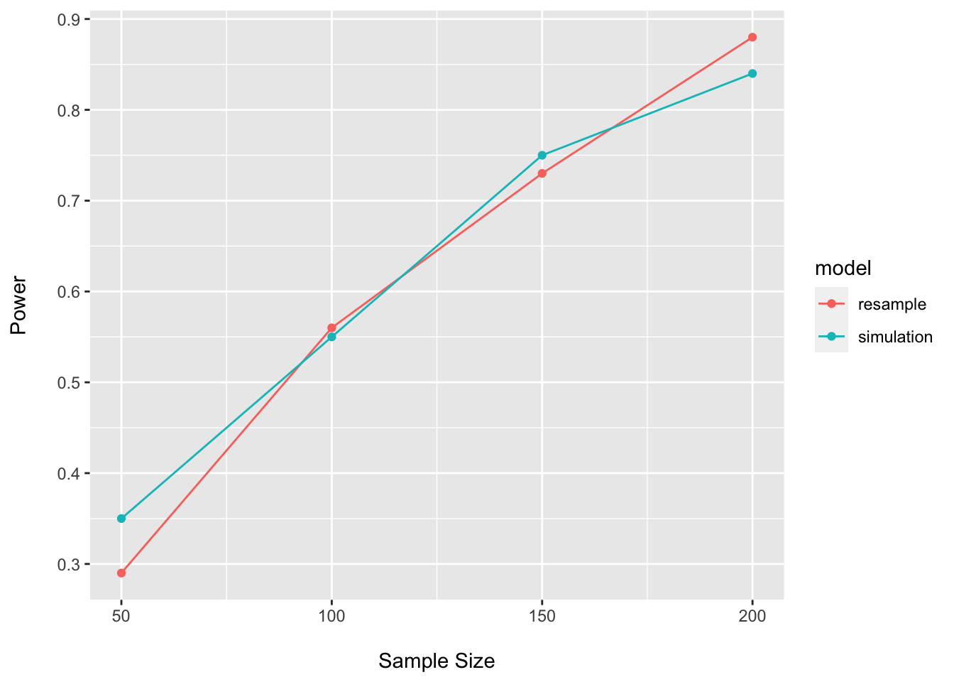
As expected, the results are quite similar for the simulation and resampling approaches.
One nice feature of the simulation approach is that it is easy to modify parameters to see how our assumptions might be impacting the results. To do this, all we need to do is try out other combinations of parameter values (i.e., assume pilot effect size may be optimistic, or our variance underestimated, etc.) and check how our estimates vary.
Here I assume a smaller effect size, and then additionally a larger variance, to generate more conservative estimates.
round(mean(replicate(1000, sim_power(sample_size = 200, log_es_t = -.6), simplify = TRUE), na.rm = TRUE), 2)## [1] 0.63round(mean(replicate(1000, sim_power(sample_size = 200, log_es_t = -.6, theta = .4), simplify = TRUE), na.rm = TRUE), 2)## [1] 0.48Assume different pilot data and data generating process
Here, as an alternative, I use the SparseDOSSA2 package to simulate the relative abundance of E.coli using the built-in stool template trained on data from the HMP. I assume a balanced design and that the relative abundance of E.coli has a -1.5 log fold change for IBD versus control.
I then fit the same ZINB regression to the data (knowing it does not match the known the DGP) and assess power at various sample sizes.
I only use n=100 replications since this function takes a bit longer to run. Be sure to use a larger number for your actual calculations.
sim_dossa <- function(sample_size, log_fold_spike){
  n_samples <- sample_size
  meta_matrix <- as.matrix(data.frame(
    row.names = paste0(rep("Sample", n_samples), 1:n_samples),
    disease = rep(c(0, 1), n_samples / 2)))

  spike_meta_df <- data.frame(
    metadata_datum = 1,
    feature_spiked = "k__Bacteria|p__Proteobacteria|c__Gammaproteobacteria|o__Enterobacteriales|f__Enterobacteriaceae|g__Escherichia|s__Escherichia_coli",
    associated_property = "abundance",
    effect_size = log_fold_spike)

  sim <- SparseDOSSA2(template = "Stool", new_features = FALSE,
                      n_sample = sample_size,
                      spike_metadata = spike_meta_df,
                      metadata_matrix = meta_matrix,
                      median_read_depth = 10000000)

  sim_df <- data.frame(sim$simulated_data)

  meta_df <- meta_matrix %>%
    data.frame(.) %>%
    mutate(seq_id = row.names(.))

  ecoli_tab <- data.frame(t(sim_df)) %>%
    select(k__Bacteria.p__Proteobacteria.c__Gammaproteobacteria.o__Enterobacteriales.f__Enterobacteriaceae.g__Escherichia.s__Escherichia_coli) %>%
    dplyr::rename("Escherichia_coli" = "k__Bacteria.p__Proteobacteria.c__Gammaproteobacteria.o__Enterobacteriales.f__Enterobacteriaceae.g__Escherichia.s__Escherichia_coli") %>%
    rownames_to_column(var = "seq_id")

  ecoli_tab <- left_join(meta_df, ecoli_tab, by = "seq_id") %>%
    select(-seq_id)

  m <- zeroinfl(Escherichia_coli ~ disease | 1, data = ecoli_tab, dist = "negbin")

  m_out <- summary(m)
  pval <- m_out$coefficients$count[2, 4]
  psig <- ifelse(pval < 0.05, 1, 0)

  return(psig)
}


dossa_power_df <- data.frame(
  n = c(50, 100, 150, 200),
  power = c(
    round(mean(replicate(100, sim_dossa(sample_size = 50, log_fold_spike = 1.5), simplify = TRUE), na.rm = TRUE), 2),
    round(mean(replicate(100, sim_dossa(sample_size = 100, log_fold_spike = 1.5), simplify = TRUE), na.rm = TRUE), 2),
    round(mean(replicate(100, sim_dossa(sample_size = 150, log_fold_spike = 1.5), simplify = TRUE), na.rm = TRUE), 2),
    round(mean(replicate(100, sim_dossa(sample_size = 200, log_fold_spike = 1.5), simplify = TRUE), na.rm = TRUE), 2)),
  model = rep(c("SparseDossa2"), 4)
)dossa_power_df## n power model
## 1 50 0.65 SparseDossa2
## 2 100 0.69 SparseDossa2
## 3 150 0.77 SparseDossa2
## 4 200 0.80 SparseDossa2power_plot <- bind_rows(power_plot, dossa_power_df)
ggplot(data = power_plot, aes(x = n, y = power, group = model, color = model)) +
geom_point() +
geom_line() +
labs(x = "\nSample Size", y = "Power\n")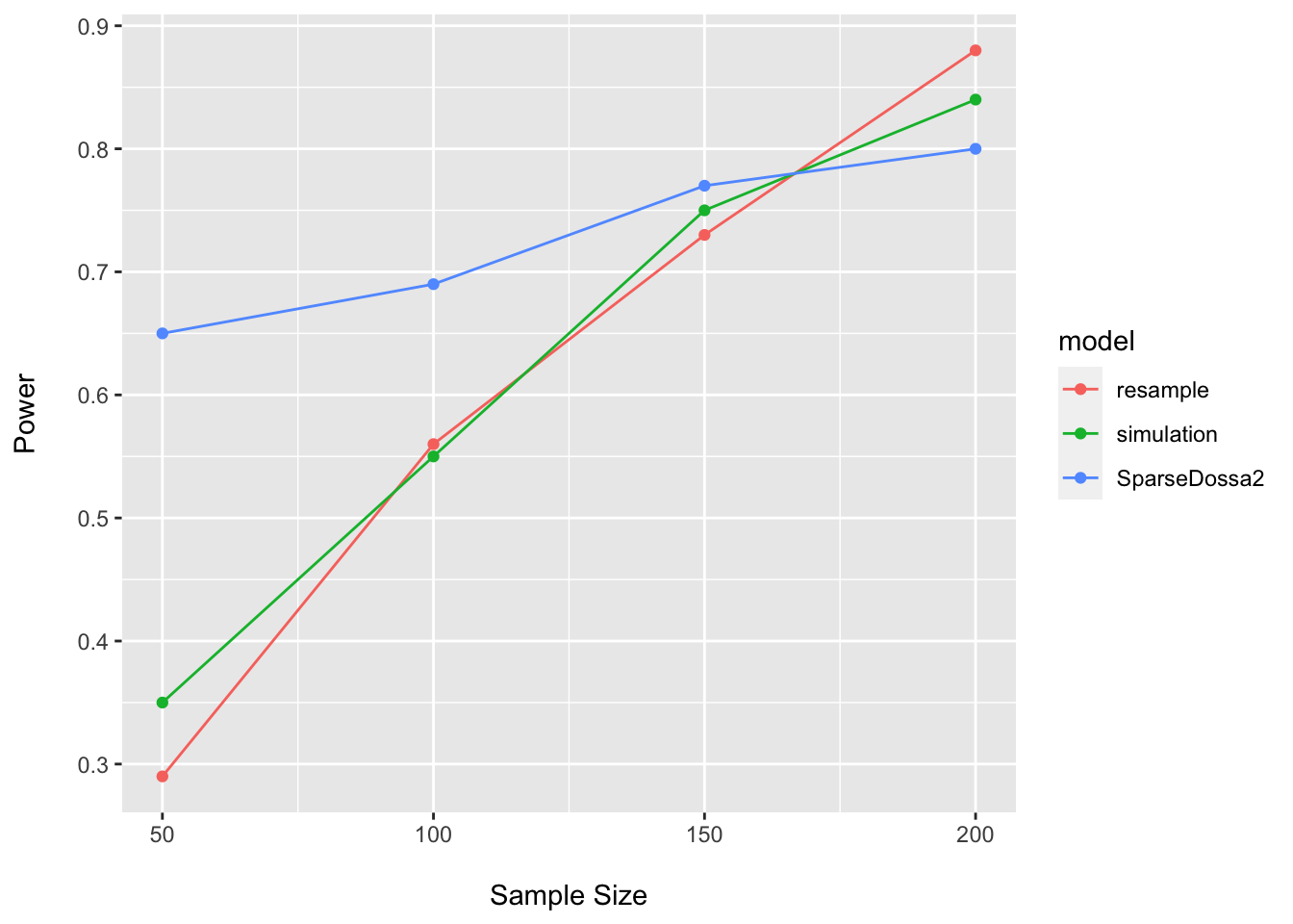
Here it is easy to see how our assumptions regarding the DGP, pilot data, assumed effect size, statistical model, etc. may all impact our estimates of power. This is one reason why such sample size calculations are inherently challenging to conduct…we never know the true process giving rise to the data (or the population parameters)…and are simply trying to make our best guess about things we cannot know with certainty.
Shannon diversity
Here I show an example of how one could power on Shannon diversity if so inclined.
I assume (for better or worse) that an independent samples t-test will be used and perform power calculations using resampling and the pwr.t.test function provided in the pwr package.
(ps_rare <- rarefy_even_depth(ps, rngseed = 243, replace = FALSE))## phyloseq-class experiment-level object
## otu_table() OTU Table: [ 264 taxa and 40 samples ]
## sample_data() Sample Data: [ 40 samples by 9 sample variables ]
## tax_table() Taxonomy Table: [ 264 taxa by 7 taxonomic ranks ]head(sample_sums(ps_rare))## CSM5MCUQ_P CSM5MCWK_P CSM79HQR_P CSM7KOTO ESM5MEEJ_P HSM5MD8A_P
## 1094292 1094292 1094292 1094292 1094292 1094292adiv_rare <- data.frame(
"Observed" = estimate_richness(ps_rare, measures = "Observed"),
"Shannon" = estimate_richness(ps_rare, measures = "Shannon"),
"disease" = sample_data(ps_rare)$disease) %>%
rownames_to_column(var = "seq_id")
head(adiv_rare)## seq_id Observed Shannon disease
## 1 CSM5MCUQ_P 78 2.718157 IBD
## 2 CSM5MCWK_P 74 2.434925 IBD
## 3 CSM79HQR_P 40 2.555218 IBD
## 4 CSM7KOTO 32 2.258737 IBD
## 5 ESM5MEEJ_P 46 2.180716 IBD
## 6 HSM5MD8A_P 96 3.043629 healthyt.test(Shannon ~ disease, data = adiv_rare)##
## Welch Two Sample t-test
##
## data: Shannon by disease
## t = 0.6529, df = 37.221, p-value = 0.5178
## alternative hypothesis: true difference in means between group healthy and group IBD is not equal to 0
## 95 percent confidence interval:
## -0.1898254 0.3703765
## sample estimates:
## mean in group healthy mean in group IBD
## 2.354850 2.264575#Resampling
boot_power_t <- function(n = 40){
boot_ids <- sample(adiv_rare$seq_id, size = n, replace = TRUE)
boot_df <- data.frame(seq_id = boot_ids)
boot_df <- left_join(boot_df, adiv_rare, by = "seq_id")
my_t <- t.test(Shannon ~ disease, data = boot_df, var.equal = TRUE)
t_out <- broom::tidy(my_t)
pval <- t_out$p.value
psig <- ifelse(pval < 0.05, 1, 0)
return(psig)
}
power_boot_t_df <- data.frame(
n = c(100, 200, 400, 800),
power = c(
round(mean(replicate(1000, boot_power_t(n = 100), simplify = TRUE)), 2),
round(mean(replicate(1000, boot_power_t(n = 200), simplify = TRUE)), 2),
round(mean(replicate(1000, boot_power_t(n = 400), simplify = TRUE)), 2),
round(mean(replicate(1000, boot_power_t(n = 800), simplify = TRUE)), 2)),
model = rep(c("resample"), 4)
)
power_boot_t_df## n power model
## 1 100 0.17 resample
## 2 200 0.30 resample
## 3 400 0.57 resample
## 4 800 0.86 resample#Closed form
adiv_rare %>%
group_by(disease) %>%
summarise(mean = mean(Shannon))## # A tibble: 2 × 2
## disease mean
## <chr> <dbl>
## 1 healthy 2.35
## 2 IBD 2.26adiv_rare %>%
summarise(sd = sd(Shannon))## sd
## 1 0.4340132(es <- round((2.35 - 2.26) / .43, 2))## [1] 0.21power_closed_t_df <- data.frame(
n = c(100, 200, 400, 800),
power = c(
round(pwr.t.test(n = 50, d = es, power = NULL, sig.level =.05, type = "two.sample", alternative = "two.sided")$power, 2),
round(pwr.t.test(n = 100, d = es, power = NULL, sig.level =.05, type = "two.sample", alternative = "two.sided")$power, 2),
round(pwr.t.test(n = 200, d = es, power = NULL, sig.level =.05, type = "two.sample", alternative = "two.sided")$power, 2),
round(pwr.t.test(n = 400, d = es, power = NULL, sig.level =.05, type = "two.sample", alternative = "two.sided")$power, 2)),
model = rep(c("formula"), 4)
)
power_closed_t_df## n power model
## 1 100 0.18 formula
## 2 200 0.32 formula
## 3 400 0.55 formula
## 4 800 0.84 formulapower_plot_t <- bind_rows(power_boot_t_df, power_closed_t_df)
ggplot(data = power_plot_t, aes(x = n, y = power, group = model, color = model)) +
geom_point() +
geom_line() +
labs(x = "\nSample Size", y = "Power\n")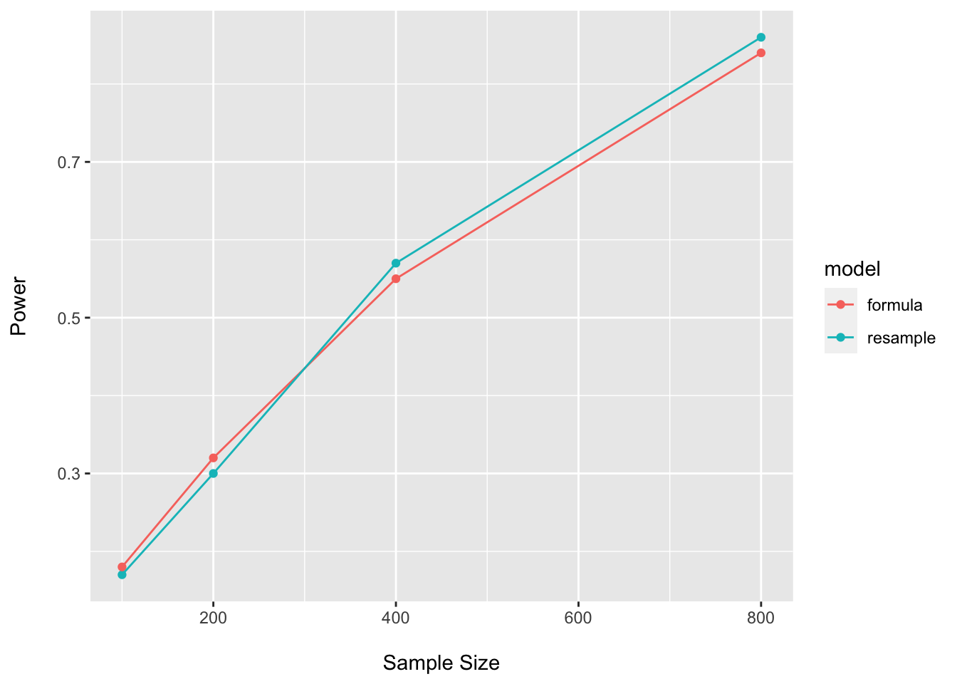
Here I am using values for the assumed effect size similar to what we see in the pilot…and we see the expected high-degree of concordance between approaches. However, it is often prudent to assume the potential for optimistic estimates in one’s pilot data and to penalize calculations accordingly.
Beta-diversity
In this section I provide some code to resample one’s pilot data and perform a power calculation for a beta-diversity PERMANOVA using the adonis function in the vegan package.
Other methods exist for beta-diversity power analyses, but to my knowledge, are specific to a few distance/dissimilarity measures. Resampling is a general approach that can be applied to any distance metric. Here I use the Aitchison distance which is the Euclidean distance after a centered log-ratio transformation of the species abundance data. Zero values are imputed with a pseudo count of one using the microbiome package to avoid division by zero.
One would also use something like spareDossa2 and generate a template for each environment and then test via simulation. However, I do not get into that here.
ps_clr <- microbiome::transform(ps, 'clr')
ord_clr <- ordinate(ps_clr, "RDA")

plot_ordination(ps_clr, ord_clr, type = "samples", color = "disease") +
    geom_point(size = 3) +
    labs(color = "Group") +
    geom_point(size = 3)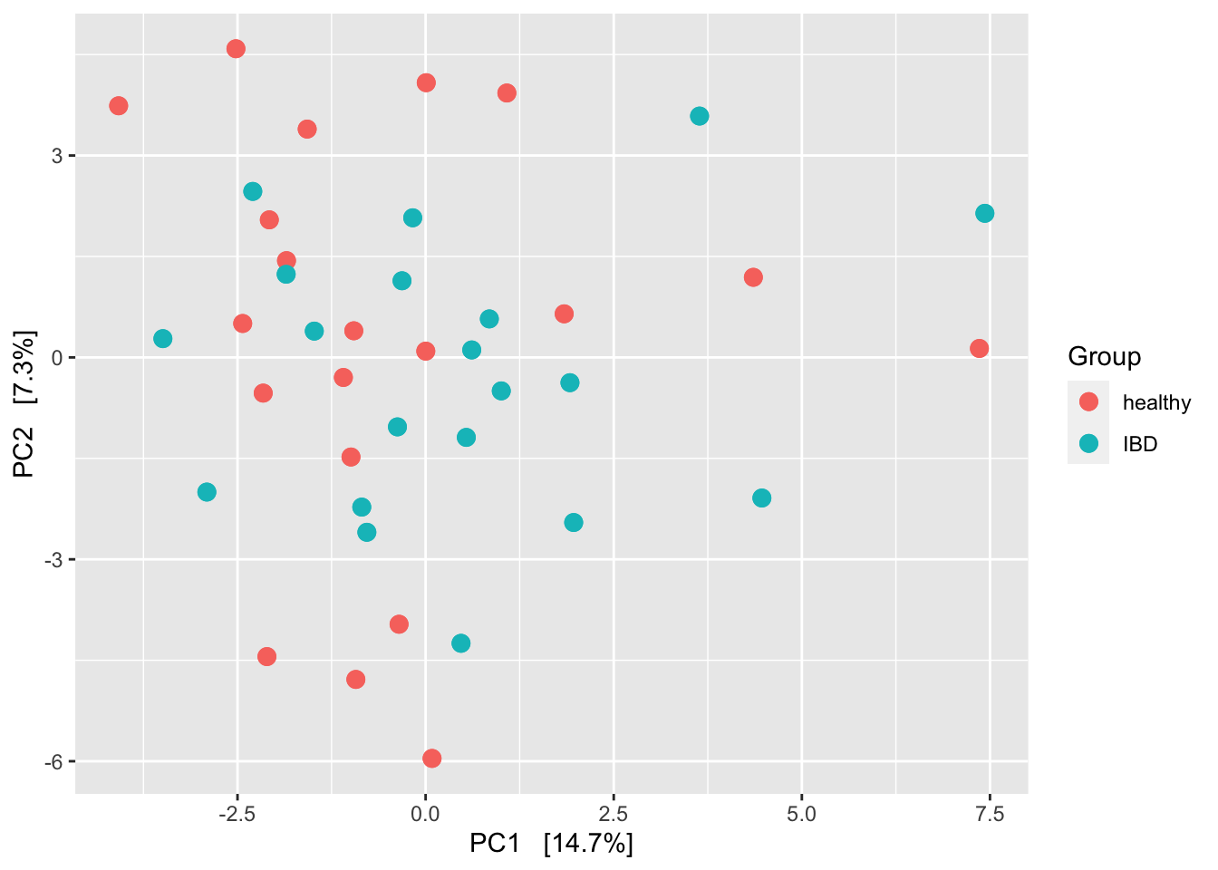
dm <- phyloseq::distance(ps_clr, "euclidean")
adonis(dm ~ sample_data(ps_clr)$disease)
##
## Call:
## adonis(formula = dm ~ sample_data(ps_clr)$disease)
##
## Permutation: free
## Number of permutations: 999
##
## Terms added sequentially (first to last)
##
## Df SumsOfSqs MeanSqs F.Model R2 Pr(>F)
## sample_data(ps_clr)$disease 1 1681 1681.3 0.95581 0.02454 0.523
## Residuals 38 66845 1759.1 0.97546
## Total 39 68526 1.00000#resampling
ps_boot <- function(ps_object = ps_clr, n_subjects = 40){
ps_ids <- sample_names(ps_object)
boot_ids <- sample(x = ps_ids, size = n_subjects, replace = TRUE)
boot_df <- data.frame(seq_id = boot_ids)
meta_df <- data.frame(sample_data(ps_object)) %>%
rownames_to_column(var = "seq_id")
join_df <- left_join(boot_df, meta_df, by = "seq_id")
otu_df <- data.frame(t(otu_table(ps_object))) %>%
rownames_to_column(var = "seq_id")
join_otu <- left_join(boot_df, otu_df, by = "seq_id")
join_df <- join_df %>%
mutate(boot_id = paste("S", row_number(), sep = "")) %>%
dplyr::select(-seq_id) %>%
column_to_rownames(var = "boot_id")
join_otu <- join_otu %>%
mutate(boot_id = paste("S", row_number(), sep = "")) %>%
dplyr::select(-seq_id) %>%
column_to_rownames(var = "boot_id") %>%
t() %>%
data.frame()
boot_ps <- phyloseq(sample_data(join_df),
otu_table(join_otu, taxa_are_rows = TRUE))
return(boot_ps)
}
permanova_fun <- function(ps_object){
my_dm <- phyloseq::distance(ps_object, "euclidean")
res <- adonis(my_dm ~ sample_data(ps_object)$disease)
pval <- res$aov.tab$`Pr(>F)`[1]
psig <- ifelse(pval < 0.05, 1, 0)
return(psig)
}
run_power <- function(sample_size = 40){
boot_ps_list <- future_replicate(n = 100, expr = ps_boot(n_subjects = sample_size), simplify = FALSE)
boot_psig <- lapply(boot_ps_list, permanova_fun)
boot_psig_df <- do.call(rbind.data.frame, boot_psig)
names(boot_psig_df) <- "p_sig"
psig <- round(mean(boot_psig_df$p_sig), 2)
return(psig)
}
plan(multisession, gc = TRUE, workers = 6)
power_boot_perm_df <- data.frame(
n = c(30, 40, 50, 60),
power = c(
run_power(sample_size = 30),
run_power(sample_size = 40),
run_power(sample_size = 50),
run_power(sample_size = 60)),
model = rep(c("resample"), 4)
)
power_boot_perm_df## n power model
## 1 30 0.53 resample
## 2 40 0.80 resample
## 3 50 0.96 resample
## 4 60 0.99 resampleggplot(data = power_boot_perm_df, aes(x = n, y = power, color = model)) +
geom_point() +
geom_line() +
labs(x = "\nSample Size", y = "Power\n")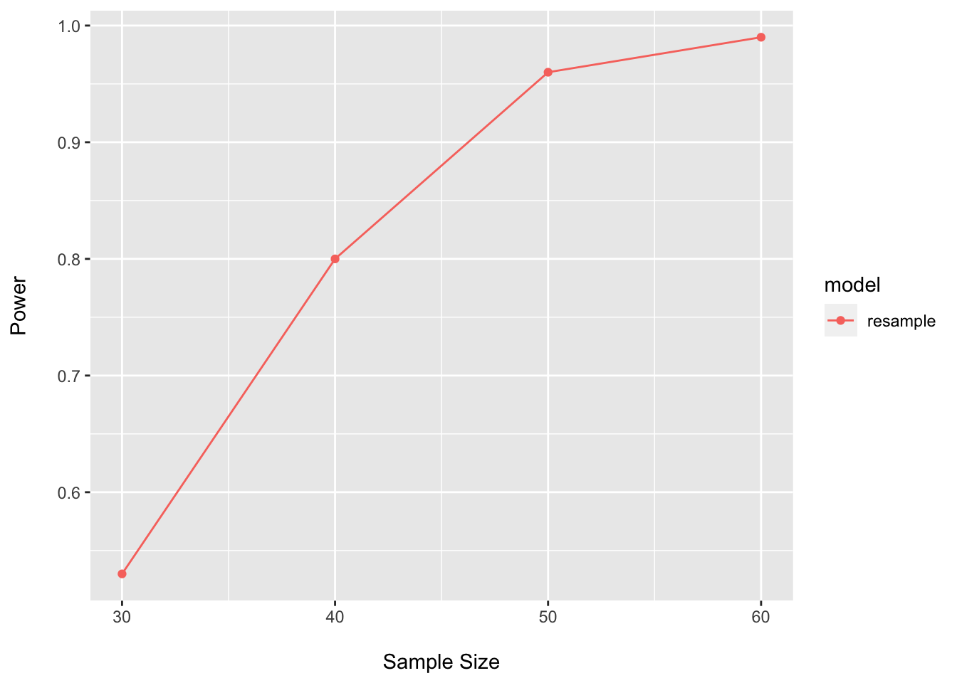
Even though there does not look to be much structure here, this tests suggests that not too many samples are needed to power on the PERMANOVA test.
Session Info
sessionInfo()## R version 4.1.1 (2021-08-10)
## Platform: x86_64-apple-darwin17.0 (64-bit)
## Running under: macOS Catalina 10.15.7
##
## Matrix products: default
## BLAS: /Library/Frameworks/R.framework/Versions/4.1/Resources/lib/libRblas.0.dylib
## LAPACK: /Library/Frameworks/R.framework/Versions/4.1/Resources/lib/libRlapack.dylib
##
## locale:
## [1] en_US.UTF-8/en_US.UTF-8/en_US.UTF-8/C/en_US.UTF-8/en_US.UTF-8
##
## attached base packages:
## [1] parallel stats4 stats graphics grDevices utils datasets
## [8] methods base
##
## other attached packages:
## [1] SparseDOSSA2_0.99.2 Rmpfr_0.8-7
## [3] gmp_0.6-2 igraph_1.2.7
## [5] truncnorm_1.0-8 magrittr_2.0.1
## [7] huge_1.3.5 mvtnorm_1.1-3
## [9] ks_1.13.3 Hmisc_4.6-0
## [11] Formula_1.2-4 survival_3.2-11
## [13] vegan_2.5-7 lattice_0.20-44
## [15] permute_0.9-5 pwr_1.3-0
## [17] broom_0.7.9 cowplot_1.1.1
## [19] future.apply_1.8.1 future_1.22.1
## [21] pscl_1.5.5 microbiome_1.14.0
## [23] phyloseq_1.36.0 curatedMetagenomicData_3.0.10
## [25] TreeSummarizedExperiment_2.0.3 Biostrings_2.60.2
## [27] XVector_0.32.0 SingleCellExperiment_1.14.1
## [29] SummarizedExperiment_1.22.0 Biobase_2.52.0
## [31] GenomicRanges_1.44.0 GenomeInfoDb_1.28.4
## [33] IRanges_2.26.0 S4Vectors_0.30.2
## [35] BiocGenerics_0.38.0 MatrixGenerics_1.4.3
## [37] matrixStats_0.61.0 forcats_0.5.1
## [39] stringr_1.4.0 dplyr_1.0.7
## [41] purrr_0.3.4 readr_2.0.2
## [43] tidyr_1.1.4 tibble_3.1.5
## [45] ggplot2_3.3.5 tidyverse_1.3.1
##
## loaded via a namespace (and not attached):
## [1] utf8_1.2.2 tidyselect_1.1.1
## [3] RSQLite_2.2.8 AnnotationDbi_1.54.1
## [5] htmlwidgets_1.5.4 grid_4.1.1
## [7] BiocParallel_1.26.2 Rtsne_0.15
## [9] munsell_0.5.0 codetools_0.2-18
## [11] withr_2.4.2 colorspace_2.0-2
## [13] filelock_1.0.2 highr_0.9
## [15] knitr_1.36 rstudioapi_0.13
## [17] listenv_0.8.0 labeling_0.4.2
## [19] GenomeInfoDbData_1.2.6 farver_2.1.0
## [21] bit64_4.0.5 rhdf5_2.36.0
## [23] parallelly_1.28.1 vctrs_0.3.8
## [25] treeio_1.16.2 generics_0.1.1
## [27] xfun_0.29 BiocFileCache_2.0.0
## [29] R6_2.5.1 bitops_1.0-7
## [31] rhdf5filters_1.4.0 cachem_1.0.6
## [33] DelayedArray_0.18.0 assertthat_0.2.1
## [35] promises_1.2.0.1 scales_1.1.1
## [37] nnet_7.3-16 gtable_0.3.0
## [39] globals_0.14.0 rlang_0.4.12
## [41] splines_4.1.1 lazyeval_0.2.2
## [43] checkmate_2.0.0 BiocManager_1.30.16
## [45] yaml_2.2.1 reshape2_1.4.4
## [47] modelr_0.1.8 backports_1.2.1
## [49] httpuv_1.6.3 tools_4.1.1
## [51] bookdown_0.24 ellipsis_0.3.2
## [53] jquerylib_0.1.4 biomformat_1.20.0
## [55] RColorBrewer_1.1-2 Rcpp_1.0.7
## [57] plyr_1.8.6 base64enc_0.1-3
## [59] zlibbioc_1.38.0 RCurl_1.98-1.5
## [61] rpart_4.1-15 haven_2.4.3
## [63] cluster_2.1.2 fs_1.5.0
## [65] data.table_1.14.2 blogdown_1.7
## [67] reprex_2.0.1 hms_1.1.1
## [69] mime_0.12 evaluate_0.14
## [71] xtable_1.8-4 jpeg_0.1-9
## [73] mclust_5.4.7 readxl_1.3.1
## [75] gridExtra_2.3 compiler_4.1.1
## [77] KernSmooth_2.23-20 crayon_1.4.1
## [79] htmltools_0.5.2 mgcv_1.8-36
## [81] later_1.3.0 tzdb_0.1.2
## [83] lubridate_1.8.0 DBI_1.1.1
## [85] ExperimentHub_2.0.0 dbplyr_2.1.1
## [87] MASS_7.3-54 rappdirs_0.3.3
## [89] Matrix_1.3-4 ade4_1.7-18
## [91] cli_3.1.0 pkgconfig_2.0.3
## [93] foreign_0.8-81 xml2_1.3.2
## [95] foreach_1.5.1 bslib_0.3.1
## [97] multtest_2.48.0 rvest_1.0.2
## [99] digest_0.6.28 pracma_2.3.3
## [101] rmarkdown_2.11 cellranger_1.1.0
## [103] tidytree_0.3.5 htmlTable_2.3.0
## [105] curl_4.3.2 shiny_1.7.1
## [107] lifecycle_1.0.1 nlme_3.1-152
## [109] jsonlite_1.7.2 Rhdf5lib_1.14.2
## [111] fansi_0.5.0 pillar_1.6.4
## [113] KEGGREST_1.32.0 fastmap_1.1.0
## [115] httr_1.4.2 interactiveDisplayBase_1.30.0
## [117] glue_1.4.2 png_0.1-7
## [119] iterators_1.0.13 BiocVersion_3.13.1
## [121] bit_4.0.4 stringi_1.7.5
## [123] sass_0.4.0 blob_1.2.2
## [125] AnnotationHub_3.0.2 latticeExtra_0.6-29
## [127] memoise_2.0.0 ape_5.5