ANCOVA for Analyzing Pre-Post Microbiome Studies
I recently analyzed some data from an experiment with a pre-post study design where our estimands of interest were the baseline adjusted mean difference in Shannon diversity and species differential abundance between arms at post-treatment. While I was able to find good software options utilizing linear mixed-effects models to test for differences in the change over time between groups (i.e., MaAsLin2, LinDA, etc.), I did not come across any that would easily allow for the inclusion of the pre-treatment microbial relative abundance data as a model covariate. So I ended up writing my own quick function to loop an analysis of covariance (ANCOVA) model over all taxa in a given dataset. I figured I would share some example code here in case it is helpful to others.
When analyzing data from a pre-post design, I typically prefer to use ANCOVA to estimate the baseline adjusted difference between groups at post-treatment. There are several reasons for this, but primary among them, is that it provides a test of the (adjusted) difference at post-treatment rather than a test of the difference in the change over time (see here for a description of Lord’s paradox if you are not familiar with the distinction between approaches). In addition, ANCOVA can provide gains in statistical power by reducing residual variance and does not take on all the “issues” associated with working with change scores. Here is a link to a paper by O’Connell et. al and one to Frank Harrell’s website that describe approaches to analyzing pre-post study designs, rational, implications, etc. in greater detail.
Since I do not own the data that served as the motivating example (i.e., cannot use and share it here), I looked through the curatedMetagenomicData package for a study with a two group, longitudinal design. I came across the study by Hall et. al. in 2017 where they collected repeated stool samples from IBD patients and otherwise healthy controls. So below I pull out data from the first and sixth visit to serve as an “example” of a pre-post microbiome study. In the future, I might return to these data to show some examples of how we could model the full longitudinal series.
The sample size here ends up being very small (i.e., at best we might view this as a pilot). So again, the focus is not on obtaining inferences from these specific data per se, but rather to use this as a didactic example highlighting how one might approach the analysis of a pre-post design. I use tidyverse syntax in most places below, and not base R (although in most of my programs I end up cobbling together a bit of both), since I find it super helpful and easier to read.
Load libraries
library(curatedMetagenomicData); packageVersion("curatedMetagenomicData") ## [1] '3.0.10'library(tidyverse); packageVersion("tidyverse") ## [1] '1.3.1'library(phyloseq); packageVersion("phyloseq") ## [1] '1.36.0'library(microbiome); packageVersion("microbiome") ## [1] '1.14.0'library(emmeans); packageVersion("emmeans") ## [1] '1.7.0'library(lmtest); packageVersion("lmtest") ## [1] '0.9.38'library(sandwich); packageVersion("sandwich") ## [1] '3.0.1'Pull curatedMetagenomicData
Here I access the sample metadata provided for the HallAB_2017 study in the curatedMetagenomicData package. Then I filter it to visit numbers 1 and 6, select the metadata columns that will be needed for the analysis, and the sample IDs we will need to pull down the correct set of taxonomic profiles.
meta_df <- curatedMetagenomicData::sampleMetadata

mydata <- meta_df %>%
  filter(study_name == "HallAB_2017") %>%
  filter(visit_number %in% c(1, 6)) %>%
  arrange(subject_id, visit_number) %>%
  select(sample_id, subject_id, visit_number, body_site, study_condition, days_from_first_collection)

count_ids <- mydata %>%
  group_by(subject_id) %>%
  summarise(n = n()) %>%
  filter(n == 2)

keep_ids <- count_ids$subject_id

mydata <- mydata %>%
  filter(subject_id %in% keep_ids) %>%
  mutate(time = ifelse(visit_number == 1, "pre", "post"),
         time = factor(time, levels = c("pre", "post")))

table(mydata$study_condition, mydata$time)
##
## pre post
## control 9 9
## IBD 15 15rm(keep_ids, count_ids)We can see that we end up with only a small number of participants with both pre and post data (9 controls and 15 IBD).
Now we can use the sample_id to pull down the species-level relative abundances (as counts) as obtained from MetaPhlAn3. I provide a bit of code to convert the SummarizedExperiment object to a phyloseq object for downstream analysis and drop some low abundance species.
keep_id <- mydata$sample_id

my_se <- sampleMetadata %>%
  dplyr::filter(sample_id %in% keep_id) %>%
  curatedMetagenomicData::returnSamples("relative_abundance", counts = TRUE)

sp_df <- as.data.frame(as.matrix(assay(my_se)))

sp_df <- sp_df %>%
  rownames_to_column(var = "Species")

otu_tab <- sp_df %>%
  tidyr::separate(Species, into = c("Kingdom", "Phylum", "Class", "Order", "Family", "Genus", "Species"), sep = "\\|") %>%
  dplyr::select(-Kingdom, -Phylum, -Class, -Order, -Family, -Genus) %>%
  dplyr::mutate(Species = gsub("s__", "", Species)) %>%
  tibble::column_to_rownames(var = "Species")

tax_tab <- sp_df %>%
  dplyr::select(Species) %>%
  tidyr::separate(Species, into = c("Kingdom", "Phylum", "Class", "Order", "Family", "Genus", "Species"), sep = "\\|") %>%
  dplyr::mutate(Kingdom = gsub("k__", "", Kingdom),
                Phylum = gsub("p__", "", Phylum),
                Class = gsub("c__", "", Class),
                Order = gsub("o__", "", Order),
                Family = gsub("f__", "", Family),
                Genus = gsub("g__", "", Genus),
                Species = gsub("s__", "", Species)) %>%
  dplyr::mutate(spec_row = Species) %>%
  tibble::column_to_rownames(var = "spec_row")

meta_df <- mydata %>%
  tibble::column_to_rownames(var = "sample_id")

(ps <- phyloseq(sample_data(meta_df),
                otu_table(otu_tab, taxa_are_rows = TRUE),
                tax_table(as.matrix(tax_tab))))
## phyloseq-class experiment-level object
## otu_table() OTU Table: [ 507 taxa and 48 samples ]
## sample_data() Sample Data: [ 48 samples by 6 sample variables ]
## tax_table() Taxonomy Table: [ 507 taxa by 7 taxonomic ranks ]minTotRelAbun <- 1e-5
x <- taxa_sums(ps)
keepTaxa <- (x / sum(x)) > minTotRelAbun
(ps <- prune_taxa(keepTaxa, ps)) ## phyloseq-class experiment-level object
## otu_table() OTU Table: [ 263 taxa and 48 samples ]
## sample_data() Sample Data: [ 48 samples by 6 sample variables ]
## tax_table() Taxonomy Table: [ 263 taxa by 7 taxonomic ranks ]rm(list= ls()[!(ls() %in% c("ps"))])We can see that we end up with data on 263 species for 48 samples.
Alpha-diversity
Here we test for differences in the baseline adjusted Shannon diversity at post-treatment. To do this, we will estimate the Shannon diversity for all participants at each time point and then fit a multiple linear regression model regressing Shannon diversity at post-treatment on an indicator variable of study_condition (i.e., IBD vs. control) and Shannon diversity at pre-treatment.
I do this after subsampling (without replacement) each sample to the same sequencing depth (for better or worse). I also provide a plot of the pre and post Shannon diversity by study condition as a means to visualize potential differences.
(ps_rare <- rarefy_even_depth(ps, rngseed = 243, replace = FALSE))## phyloseq-class experiment-level object
## otu_table() OTU Table: [ 263 taxa and 48 samples ]
## sample_data() Sample Data: [ 48 samples by 6 sample variables ]
## tax_table() Taxonomy Table: [ 263 taxa by 7 taxonomic ranks ]head(sample_sums(ps_rare))## SKST006_6_G102964 SKST006_1_G102959 SKST027_6_G102955 SKST027_1_G102984
## 178064 178064 178064 178064
## SKST014_6_G102951 SKST023_1_G102981
## 178064 178064adiv <- data.frame(
"Shannon" = estimate_richness(ps_rare, measures = "Shannon"),
"id" = sample_data(ps_rare)$subject_id,
"time" = sample_data(ps_rare)$time,
"study_condition" = sample_data(ps_rare)$study_condition)
head(adiv)## Shannon id time study_condition
## SKST006_6_G102964 1.542647 SKST006 post IBD
## SKST006_1_G102959 1.802048 SKST006 pre IBD
## SKST027_6_G102955 1.115893 SKST027 post IBD
## SKST027_1_G102984 1.232501 SKST027 pre IBD
## SKST014_6_G102951 2.485732 SKST014 post IBD
## SKST023_1_G102981 2.043091 SKST023 pre controlggplot(data = adiv, aes(x = time, y = Shannon, group = id, color = id)) +
geom_point() +
geom_line() +
facet_grid(~study_condition) +
labs(x = "", y = "Shannon Diversity\n") +
theme(legend.position = "none")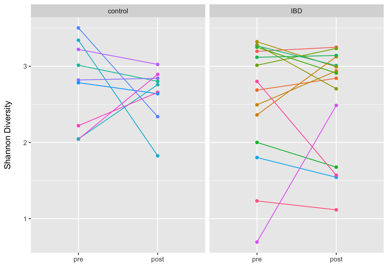
Next we convert the data from long to wide format for analysis using the pivot_wider function and fit the ANCOVA model via multiple linear regression. I also provide some code to obtain the estimated marginal means (i.e., least squares means) for each group at follow-up.
adiv_wide <- adiv %>%
  pivot_wider(names_from = time, values_from = c(Shannon))

m1 <- lm(post ~ study_condition + pre, data = adiv_wide)
summary(m1)
##
## Call:
## lm(formula = post ~ study_condition + pre, data = adiv_wide)
##
## Residuals:
## Min 1Q Median 3Q Max
## -1.0840 -0.2368 0.1841 0.3865 0.6312
##
## Coefficients:
## Estimate Std. Error t value Pr(>|t|)
## (Intercept) 1.625254 0.495059 3.283 0.00355 **
## study_conditionIBD 0.003171 0.240623 0.013 0.98961
## pre 0.366218 0.164894 2.221 0.03749 *
## ---
## Signif. codes: 0 '***' 0.001 '**' 0.01 '*' 0.05 '.' 0.1 ' ' 1
##
## Residual standard error: 0.5648 on 21 degrees of freedom
## Multiple R-squared: 0.1932, Adjusted R-squared: 0.1163
## F-statistic: 2.514 on 2 and 21 DF, p-value: 0.105par(mfrow=c(2,2)); plot(m1); par(mfrow=c(1,1))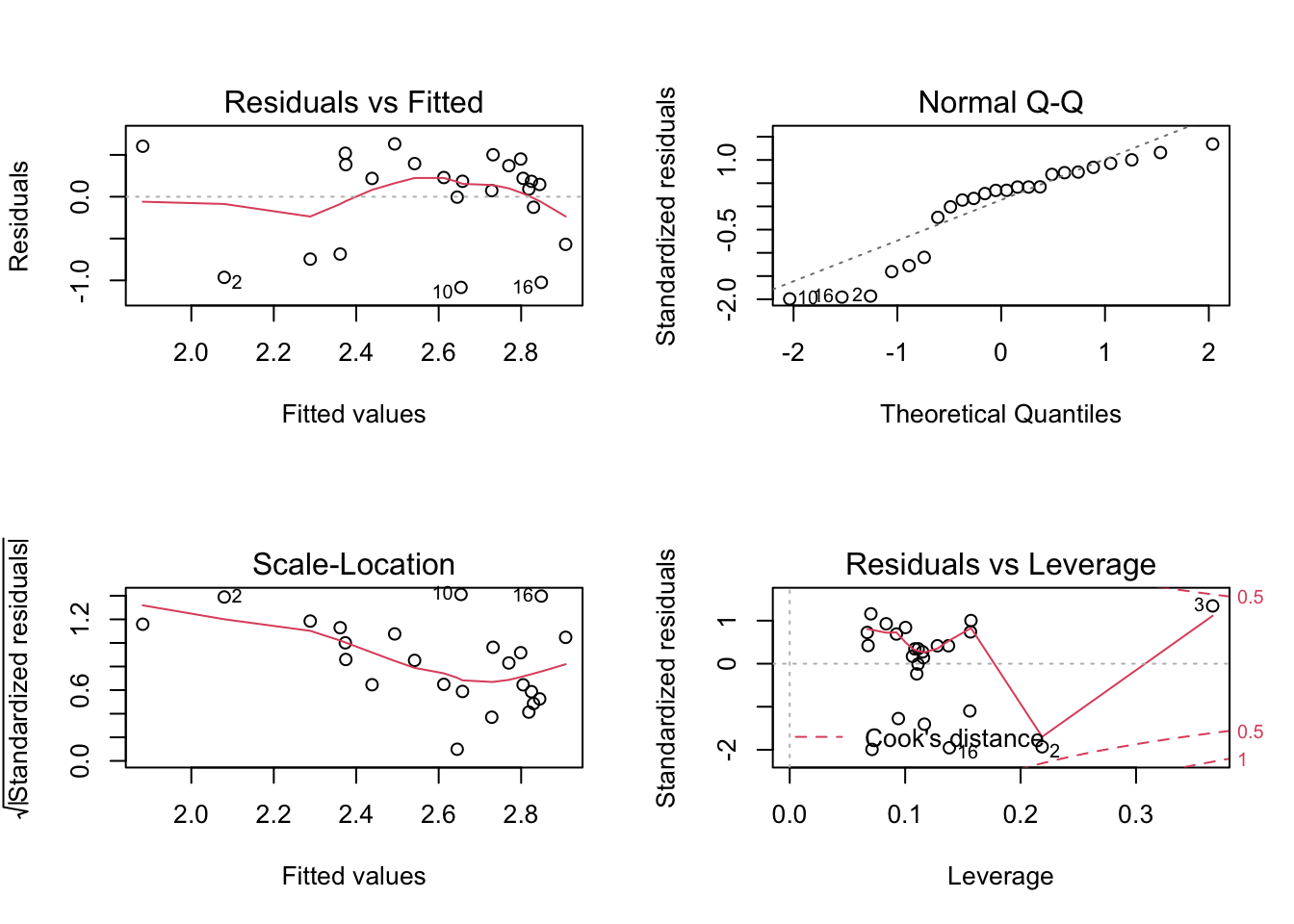
em1 <- emmeans(m1,  ~ study_condition + pre)
em1_df <- as.data.frame(em1)
ggplot(data = em1_df, aes(x = study_condition, y = emmean, colour = study_condition)) +
    geom_errorbar(aes(ymin = lower.CL, ymax = upper.CL), width=.1) +
    geom_point() +
    labs(x = "", y = "Shannon Diversity\n") +
    theme(legend.position = "none")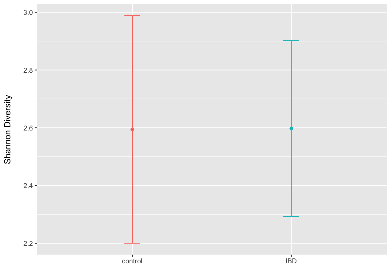
rm(m1, adiv, adiv_wide, em1, em1_df)Overall, we do not see any indication that the Shannon diversity differs on average for the IBD patients when compared to controls after adjusting for baseline values.
The model fit is perhaps sub-optimal (i.e., we likely need the residual distribution to be approximately normally distributed to make valid inferences given the small sample size). Thus, here you might want to try some transformations to see if the fit could be improved (with the issues that come along with such a transformation) or perhaps consider another approach such as an ordinal cumulative probability model for a continuous response (the rms::orm function is my go to).
Beta-diversity
I am not sure there is a good way to obtain a baseline adjusted difference for a given beta-diversity metric since by definition we are comparing the distance/dissimilarity for two samples. Thus, what I tend to do here is use the approach of first-distances I first saw described by Nicholas Bokulich et. al. and available in the QIIME2 longitudinal plug-in. Here we compute the within-subject distance/dissimilarity for paired samples and then just test for the difference between groups. Of course this is more akin to assessing “differences in change”, but at current I do not have any better ideas (please shoot me an email if you do).
First we generate a principal coordinates ordination of the Bray-Curtis dissimilarity and annotate it by study condition and time point. Then we hop through some code to obtain a data.frame of pairwise Bray-Curtis dissimilarities, plot them by condition, and do some formal testing (t-test and Wilcoxon rank-sum).
ord_bray <- ordinate(ps_rare, method = "PCoA", distance = "bray")

plot_ordination(ps_rare, ord_bray, type = "samples", color = "study_condition", shape = "time") +
  geom_point(size = 3) +
  labs(color = "Study\nCondition", shape = "Time")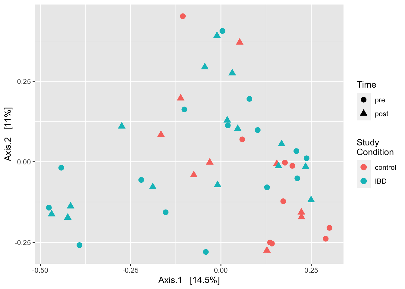
dm <- phyloseq::distance(ps_rare, method = "bray")
bray_df <- reshape2::melt(as.matrix(dm), varnames = c("s1", "s2"))

bray_df <- bray_df %>%
  separate(s1, into = c("id_1", "sample_1", "post"), sep = "_", remove = FALSE) %>%
  separate(s2, into = c("id_2", "sample_2", "post"), sep = "_", remove = FALSE) %>%
  mutate(sample_1 = ifelse(sample_1 == "mo1", 1, ifelse(sample_1 == "mo6", 6, sample_1)),
         sample_2 = ifelse(sample_2 == "mo1", 1, ifelse(sample_2 == "mo6", 6, sample_2))) %>%
  filter(id_1 == id_2) %>%
  filter(sample_1 == 1) %>%
  filter(sample_2 == 6) %>%
  dplyr::select(id_1, value) %>%
  dplyr::rename("subject_id" = "id_1",
                "within_subject_bc" = "value")

meta_df <- data.frame(sample_data(ps_rare)) %>%
  filter(time == "pre") %>%
  dplyr::select(subject_id, study_condition)

bray_df <- left_join(bray_df, meta_df)
head(bray_df)
## subject_id within_subject_bc study_condition
## 1 SKST006 0.9991632 IBD
## 2 SKST027 1.0000000 IBD
## 3 SKST014 0.9998203 IBD
## 4 SKST010 0.6000595 control
## 5 SKST023 0.8289604 control
## 6 SKST024 0.7396554 controlggplot(data = bray_df, aes(x = study_condition, y = within_subject_bc)) +
geom_boxplot(outlier.shape = NA) +
geom_jitter(height = 0, width = .2, aes(color = study_condition)) +
labs(x = "", y = "Bray-Curtis Dissimilarity\n") +
theme(legend.position = "none") +
ggtitle("First-Distances")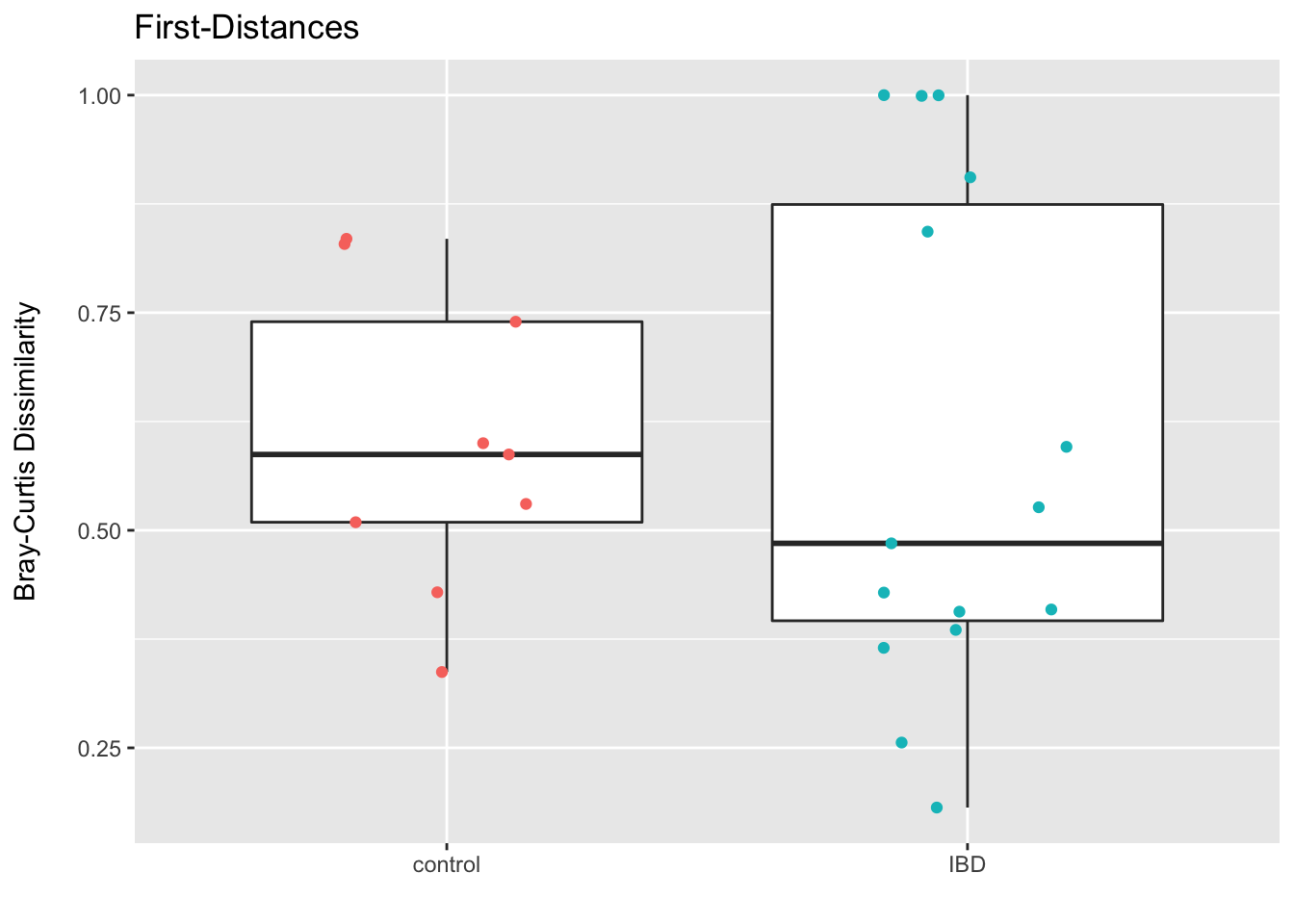
t.test(within_subject_bc ~ study_condition, data = bray_df)##
## Welch Two Sample t-test
##
## data: within_subject_bc by study_condition
## t = 0.14708, df = 21.98, p-value = 0.8844
## alternative hypothesis: true difference in means between group control and group IBD is not equal to 0
## 95 percent confidence interval:
## -0.1804498 0.2079972
## sample estimates:
## mean in group control mean in group IBD
## 0.5995803 0.5858066wilcox.test(within_subject_bc ~ study_condition, data = bray_df)##
## Wilcoxon rank sum exact test
##
## data: within_subject_bc by study_condition
## W = 75, p-value = 0.6824
## alternative hypothesis: true location shift is not equal to 0rm(bray_df, ord_bray, m1, meta_df, dm)The plot and tests do not suggests a clear difference in the change in dissimilarity from baseline for those with IBD when compared to controls. If anything, I would be interested in trying to understand if any of the sample meta (including the set up and sequencing info etc) helped explain the subset of those with IBD and very high dissimilarities. My intuition is to view such high values as suspect (I would also check the extent to which the sub-sampling might be impacting the results…or if I misunderstood the how the subject ID was being retained in the sample_id field and have some people mixed up).
Differential abundance testing
Here our goal is to obtain the baseline adjusted difference in the relative abundance of each species (for better or worse). To do this, we first centered log-ratio transform the relative abundances to account for the compositional nature of the sequence data (great explanation as to why provided by Thomas Quinn et. al) and filter out low prevalence species.
Then we write a function to fit the ANCOVA model via robust multiple linear regression where the default HC3 method of the sandwich::vcovHC function is used to obtain robust standard errors. We use robust regression here in the hopes that it will provide us more accurate standard errors in the presence of non-constant variance (which we might assume to occur for some taxa, but will not be able to check when fitting this many models). One downside is that we lose power when the variance is constant. Other options might be to trim outliers (i.e, Windsor) or to rely on the central limit theorem when the sample size is large.
We use the tidyverse nest and purr functions to nest the data for each species into its own data.frame then to loop the function over each data.frame and convert the results to the log2 fold scale for compatibility with other DA approaches.
(ps_clr <- transform(ps, transform = "clr"))## phyloseq-class experiment-level object
## otu_table() OTU Table: [ 263 taxa and 48 samples ]
## sample_data() Sample Data: [ 48 samples by 6 sample variables ]
## tax_table() Taxonomy Table: [ 263 taxa by 7 taxonomic ranks ](ps_filt <- filter_taxa(ps, function(x) sum(x > 0) > (0.3*length(x)), TRUE)) ## phyloseq-class experiment-level object
## otu_table() OTU Table: [ 94 taxa and 48 samples ]
## sample_data() Sample Data: [ 48 samples by 6 sample variables ]
## tax_table() Taxonomy Table: [ 94 taxa by 7 taxonomic ranks ]keep_taxa <- taxa_names(ps_filt)
(ps_clr_filt <- prune_taxa(keep_taxa, ps_clr))## phyloseq-class experiment-level object
## otu_table() OTU Table: [ 94 taxa and 48 samples ]
## sample_data() Sample Data: [ 48 samples by 6 sample variables ]
## tax_table() Taxonomy Table: [ 94 taxa by 7 taxonomic ranks ]my_otus <- data.frame(t(data.frame(otu_table(ps_clr_filt))))
my_otus <- my_otus %>%
rownames_to_column(var = "seq_id")
meta_df <- data.frame(sample_data(ps_clr_filt)) %>%
rownames_to_column(var = "seq_id") %>%
dplyr::select(seq_id, subject_id, study_condition, time)
clr_df <- left_join(meta_df, my_otus) %>%
dplyr::select(-seq_id) %>%
pivot_longer(cols = c(-subject_id, -study_condition, -time), names_to = "species", values_to = "abundance") %>%
arrange(species, subject_id, time)
robust_lm <- function(my_df){
df <- pivot_wider(data = my_df, names_from = time, values_from = abundance)
m <- lm(post ~ study_condition + pre, data = df)
m_out <- data.frame(t(data.frame(coeftest(m, vcov. = vcovHC(m))[2, ])))
return(m_out)
}
res_df <- clr_df %>%
tidyr::nest(data = c(-species)) %>%
dplyr::mutate(model = map(data, ~ robust_lm(my_df = .))) %>%
select(-data) %>%
unnest(cols = c(model)) %>%
dplyr::rename("se" = "Std..Error", "p.value" = "Pr...t..") %>%
rename_all(tolower) %>%
arrange(p.value) %>%
mutate(padj = p.adjust(p.value, method = "fdr"),
log2FoldChange = log2(exp(estimate)),
se = log2(exp(se))) %>%
dplyr::select(species, log2FoldChange, se, t.value, p.value, padj)
head(res_df, 10)## # A tibble: 10 × 6
## species log2FoldChange se t.value p.value padj
## <chr> <dbl> <dbl> <dbl> <dbl> <dbl>
## 1 Intestinibacter_bartlettii 3.95 1.23 3.22 0.00412 0.387
## 2 Lawsonibacter_asaccharolyticus 4.85 1.79 2.70 0.0133 0.475
## 3 Bacteroides_fragilis -7.83 2.96 -2.64 0.0152 0.475
## 4 Holdemania_filiformis -3.72 1.73 -2.15 0.0434 0.888
## 5 Bacteroides_caccae 2.96 1.47 2.02 0.0561 0.888
## 6 Enterorhabdus_caecimuris 2.79 1.43 1.95 0.0644 0.888
## 7 Roseburia_sp_CAG_471 2.34 1.24 1.89 0.0730 0.888
## 8 Clostridium_lavalense 3.09 1.66 1.86 0.0766 0.888
## 9 Eubacterium_sp_CAG_38 4.97 2.81 1.77 0.0917 0.888
## 10 Fusicatenibacter_saccharivorans -3.65 2.14 -1.71 0.103 0.888Above we can see the top ranked species according the the p-value and FDR p-value. Typically, if we purse DA testing, the information in this table is generally what we are interested in.
Below is come code to plot the results for the top taxa.
ggplot(data = filter(res_df, p.value < .1), aes(x = species, y = log2FoldChange)) +
    geom_col(alpha = .8, fill = "dodgerblue") +
    labs(y = "\nLog2 Fold-Change", x = "") +
    theme(axis.text.x = element_text(color = "black", size = 8),
          axis.text.y = element_text(color = "black", size = 8),
          axis.title.y = element_text(size = 8),
          axis.title.x = element_text(size = 10),
          legend.text = element_text(size = 8),
          legend.title = element_text(size = 8)) +
    coord_flip() +
    geom_hline(yintercept = 0, linetype="dotted") +
    theme(legend.position = "none")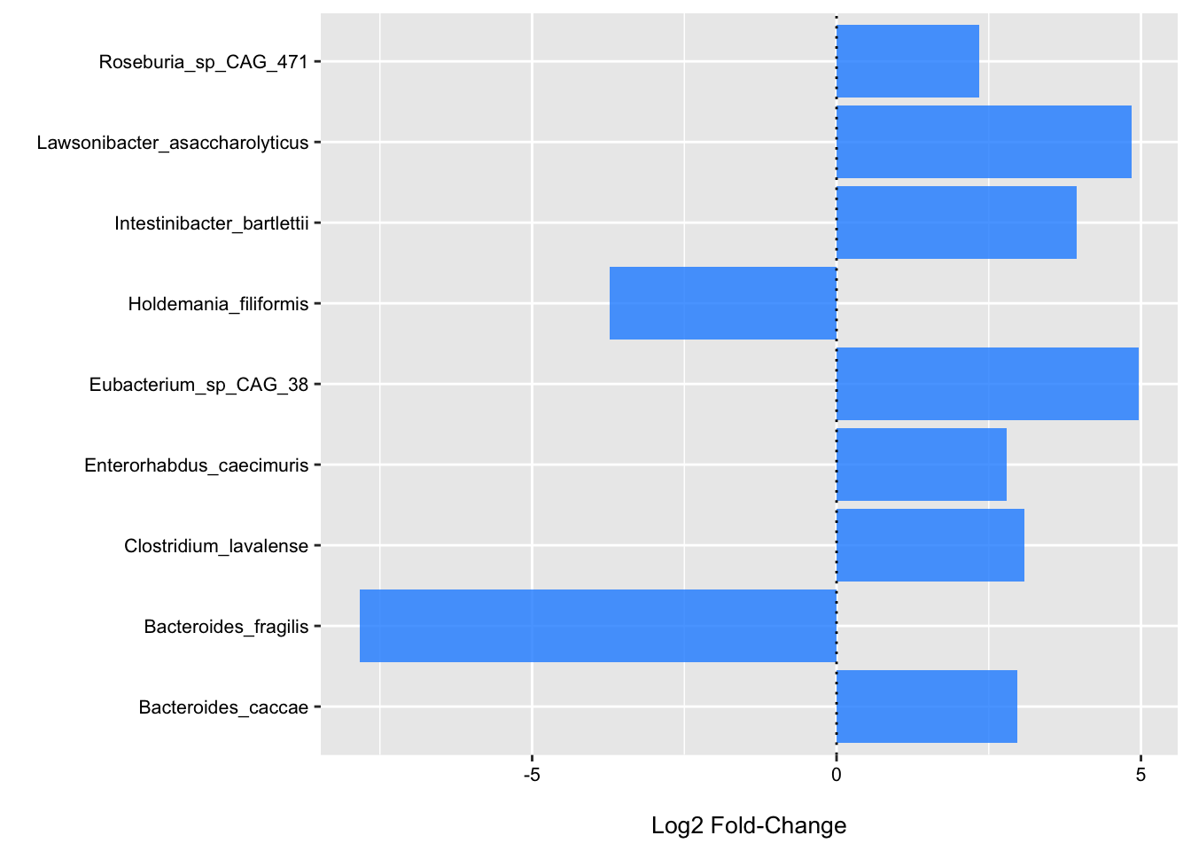
Session Info
sessionInfo()## R version 4.1.1 (2021-08-10)
## Platform: x86_64-apple-darwin17.0 (64-bit)
## Running under: macOS Catalina 10.15.7
##
## Matrix products: default
## BLAS: /Library/Frameworks/R.framework/Versions/4.1/Resources/lib/libRblas.0.dylib
## LAPACK: /Library/Frameworks/R.framework/Versions/4.1/Resources/lib/libRlapack.dylib
##
## locale:
## [1] en_US.UTF-8/en_US.UTF-8/en_US.UTF-8/C/en_US.UTF-8/en_US.UTF-8
##
## attached base packages:
## [1] parallel stats4 stats graphics grDevices utils datasets
## [8] methods base
##
## other attached packages:
## [1] sandwich_3.0-1 lmtest_0.9-38
## [3] zoo_1.8-9 emmeans_1.7.0
## [5] microbiome_1.14.0 phyloseq_1.36.0
## [7] forcats_0.5.1 stringr_1.4.0
## [9] dplyr_1.0.7 purrr_0.3.4
## [11] readr_2.0.2 tidyr_1.1.4
## [13] tibble_3.1.5 ggplot2_3.3.5
## [15] tidyverse_1.3.1 curatedMetagenomicData_3.0.10
## [17] TreeSummarizedExperiment_2.0.3 Biostrings_2.60.2
## [19] XVector_0.32.0 SingleCellExperiment_1.14.1
## [21] SummarizedExperiment_1.22.0 Biobase_2.52.0
## [23] GenomicRanges_1.44.0 GenomeInfoDb_1.28.4
## [25] IRanges_2.26.0 S4Vectors_0.30.2
## [27] BiocGenerics_0.38.0 MatrixGenerics_1.4.3
## [29] matrixStats_0.61.0
##
## loaded via a namespace (and not attached):
## [1] readxl_1.3.1 backports_1.2.1
## [3] AnnotationHub_3.0.2 BiocFileCache_2.0.0
## [5] plyr_1.8.6 igraph_1.2.7
## [7] lazyeval_0.2.2 splines_4.1.1
## [9] BiocParallel_1.26.2 TH.data_1.1-0
## [11] digest_0.6.28 foreach_1.5.1
## [13] htmltools_0.5.2 fansi_0.5.0
## [15] magrittr_2.0.1 memoise_2.0.0
## [17] cluster_2.1.2 tzdb_0.1.2
## [19] modelr_0.1.8 colorspace_2.0-2
## [21] blob_1.2.2 rvest_1.0.2
## [23] rappdirs_0.3.3 haven_2.4.3
## [25] xfun_0.29 crayon_1.4.1
## [27] RCurl_1.98-1.5 jsonlite_1.7.2
## [29] survival_3.2-11 iterators_1.0.13
## [31] ape_5.5 glue_1.4.2
## [33] gtable_0.3.0 zlibbioc_1.38.0
## [35] DelayedArray_0.18.0 Rhdf5lib_1.14.2
## [37] scales_1.1.1 mvtnorm_1.1-3
## [39] DBI_1.1.1 Rcpp_1.0.7
## [41] xtable_1.8-4 tidytree_0.3.5
## [43] bit_4.0.4 httr_1.4.2
## [45] ellipsis_0.3.2 farver_2.1.0
## [47] pkgconfig_2.0.3 sass_0.4.0
## [49] dbplyr_2.1.1 utf8_1.2.2
## [51] labeling_0.4.2 tidyselect_1.1.1
## [53] rlang_0.4.12 reshape2_1.4.4
## [55] later_1.3.0 AnnotationDbi_1.54.1
## [57] munsell_0.5.0 BiocVersion_3.13.1
## [59] cellranger_1.1.0 tools_4.1.1
## [61] cachem_1.0.6 cli_3.1.0
## [63] generics_0.1.1 RSQLite_2.2.8
## [65] ExperimentHub_2.0.0 ade4_1.7-18
## [67] broom_0.7.9 evaluate_0.14
## [69] biomformat_1.20.0 fastmap_1.1.0
## [71] yaml_2.2.1 knitr_1.36
## [73] bit64_4.0.5 fs_1.5.0
## [75] KEGGREST_1.32.0 nlme_3.1-152
## [77] mime_0.12 xml2_1.3.2
## [79] compiler_4.1.1 rstudioapi_0.13
## [81] filelock_1.0.2 curl_4.3.2
## [83] png_0.1-7 interactiveDisplayBase_1.30.0
## [85] reprex_2.0.1 treeio_1.16.2
## [87] bslib_0.3.1 stringi_1.7.5
## [89] highr_0.9 blogdown_1.7
## [91] lattice_0.20-44 Matrix_1.3-4
## [93] vegan_2.5-7 permute_0.9-5
## [95] multtest_2.48.0 vctrs_0.3.8
## [97] pillar_1.6.4 lifecycle_1.0.1
## [99] rhdf5filters_1.4.0 BiocManager_1.30.16
## [101] jquerylib_0.1.4 estimability_1.3
## [103] data.table_1.14.2 bitops_1.0-7
## [105] httpuv_1.6.3 R6_2.5.1
## [107] bookdown_0.24 promises_1.2.0.1
## [109] codetools_0.2-18 MASS_7.3-54
## [111] assertthat_0.2.1 rhdf5_2.36.0
## [113] withr_2.4.2 multcomp_1.4-17
## [115] GenomeInfoDbData_1.2.6 mgcv_1.8-36
## [117] hms_1.1.1 grid_4.1.1
## [119] coda_0.19-4 rmarkdown_2.11
## [121] Rtsne_0.15 shiny_1.7.1
## [123] lubridate_1.8.0