Identifying Differentially Abundant Features in Microbiome Data
A common goal in many microbiome studies is to identify features (i.e., species, OTUs, gene families, etc.) that differ according to some study condition of interest. While often done, this is a difficult task, and in the Introduction to the Statistical Analysis of Microbiome Data in R post I touch on some of the reasons for this. Aspects of microbiome count matrices, whether taxonomic or functional, that cause difficulties include:
- the high dimensional set of features (often 100s to 10,000s of features)
- high degree of sparsity (many features seen in only a few samples)
- complex correlation structure among features
- compositional nature of returned counts (i.e., observed counts constrained by total library size)
- differing library sizes
- over-dispersed counts
- etc.
Ultimately, as pointed out by Douglas and Langille in a recent pre-print, no parametric distribution is likely optimal for all taxa leading to modeling approaches often failing to control the type I error rate under the null hypothesis or in excessive false positive findings. These results have been observed in multiple papers using various strategies to simulate microbiome datasets with known properties. The pre-print I link to above cites a few of these papers…and I recommend you give them a read if you are not already familiar with this literature.
So then I am often asked "how does one proceed to identity differentially abundant features if there is no clear best modeling approach? One approach might be to consider the available options and decide if one approach is perhaps best suited for your particular purposes and dataset. However, this is often unclear. So I typically like to consider a few different models that seem reasonable for the data at hand and then prioritize the set of DA features called by multiple approaches. While this is imperfect, it provides some confidence that the results are at least robust to the modeling choice and may help to identify those features that seem to be changing most in relative abundance.
Below I show an example of fitting five different models to identity differentially abundant species from shotgun metagenomic data classified using MetaPhlAn2. These approaches can also be applied (perhaps more suited) to ASVs or OTUs classified via amplicon sequencing. I selected these methods because they: have performed well in one or more simulation studies, can accommodate covariate adjustment, perform formal testing, provide a diverse range of normalization and modeling approaches (i.e., count-based vs. compositional, negative binomial vs. linear model, etc.), are commonly used/popular, and are available in R. There are other good choices in both R and QIIME2 and this set is not meant to be seen as exhaustive. The models fit below include:
We will use publicly available provided by the curatedMetagenomicData package to identify differentially abudnant species in stool samples collected from participants in Southern India (Kerala) compared to North-Central India (Bhopal). The study described by Dhakhan et. al. can be found here. First we import the data, do a little clean up, fit the models, and assess the overlap in feature sets.
Loading required libraries
library(curatedMetagenomicData); packageVersion("curatedMetagenomicData") ## [1] '1.18.2'library(tidyverse); packageVersion("tidyverse") ## [1] '1.3.0'library(phyloseq); packageVersion("phyloseq") ## [1] '1.32.0'library(edgeR); packageVersion("edgeR") ## [1] '3.30.3'library(limma); packageVersion("limma") ## [1] '3.44.3'library(DEFormats); packageVersion("DEFormats") ## [1] '1.18.0'library(DESeq2); packageVersion("DESeq2") ## [1] '1.28.1'library(apeglm); packageVersion("apeglm") ## [1] '1.10.0'library(corncob); packageVersion("corncob") ## [1] '0.1.0'library(ANCOMBC); packageVersion("ANCOMBC") ## [1] '1.0.3'library(Maaslin2); packageVersion("Maaslin2") ## [1] '1.2.0'library(VennDiagram); packageVersion("VennDiagram") ## [1] '1.6.20'Grabbing the Dhakan data
dhakan_eset <- DhakanDB_2019.metaphlan_bugs_list.stool()## snapshotDate(): 2020-04-27## see ?curatedMetagenomicData and browseVignettes('curatedMetagenomicData') for documentation## loading from cache(ps <- ExpressionSet2phyloseq(dhakan_eset,
simplify = TRUE,
relab = FALSE,
phylogenetictree = FALSE))## phyloseq-class experiment-level object
## otu_table() OTU Table: [ 768 taxa and 110 samples ]
## sample_data() Sample Data: [ 110 samples by 20 sample variables ]
## tax_table() Taxonomy Table: [ 768 taxa by 8 taxonomic ranks ](ps <- subset_taxa(ps, !is.na(Species) & is.na(Strain)))## phyloseq-class experiment-level object
## otu_table() OTU Table: [ 286 taxa and 110 samples ]
## sample_data() Sample Data: [ 110 samples by 20 sample variables ]
## tax_table() Taxonomy Table: [ 286 taxa by 8 taxonomic ranks ]taxa_names(ps) <- gsub("s__", "", taxa_names(ps)) #removing s__ in OTU names)
head(taxa_names(ps))## [1] "Prevotella_copri" "Eubacterium_rectale"
## [3] "Butyrivibrio_crossotus" "Prevotella_stercorea"
## [5] "Faecalibacterium_prausnitzii" "Subdoligranulum_unclassified"(ps <- filter_taxa(ps, function(x) sum(x > 0) > (0.1*length(x)), TRUE)) #removing species not seen > 10% of samples## phyloseq-class experiment-level object
## otu_table() OTU Table: [ 109 taxa and 110 samples ]
## sample_data() Sample Data: [ 110 samples by 20 sample variables ]
## tax_table() Taxonomy Table: [ 109 taxa by 8 taxonomic ranks ]head(sort(sample_sums(ps))) #min seq depth looks good## DHAK_HV DHAK_HW DHAK_HBR DHAK_HDB DHAK_HBC DHAK_HCB
## 3829049 3843027 4216987 4683683 4689086 4820514sample_variables(ps)## [1] "subjectID" "body_site"
## [3] "antibiotics_current_use" "study_condition"
## [5] "disease" "age"
## [7] "infant_age" "age_category"
## [9] "gender" "BMI"
## [11] "country" "location"
## [13] "non_westernized" "DNA_extraction_kit"
## [15] "number_reads" "number_bases"
## [17] "minimum_read_length" "median_read_length"
## [19] "curator" "NCBI_accession"sample_data(ps)$location <- factor(sample_data(ps)$location, levels = c("Bhopal", "Kerala"))
table(sample_data(ps)$location) ##
## Bhopal Kerala
## 53 57We now have a phyloseq object with 109 species after filtering low prevalence taxa and samples from n=53 participants in Bhopal and n=57 in Kerala. I typically tend to filter out features seen in fewer than 10% to 50% of samples depending on the overall number and sparsity to better meet model assumptions and limit the FDR penalty paid when testing lower powered taxa seen in a small number of samples. Many/most tools will do this by default and provide user modifiable settings. A total of 109 species is certainly on the low side, but will allow us to quickly run these examples.
Limma-Voom with TMM normalization
dds <- phyloseq_to_deseq2(ps, ~ location) #convert to DESeq2 and DGEList objects## converting counts to integer modedge <- as.DGEList(dds)
dge <- calcNormFactors(dge, method = "TMM") #store TMM norm factor
head(dge$samples$norm.factors)## [1] 0.4529756 1.6721557 0.1509053 0.4569702 0.4646246 0.3362776mm <- model.matrix(~ group, dge$samples) #construct model matrix
head(mm)## (Intercept) groupKerala
## DHAK_HAK 1 0
## DHAK_HAJ 1 0
## DHAK_HAI 1 0
## DHAK_HAH 1 0
## DHAK_HAG 1 0
## DHAK_HAF 1 0table(mm[, 2])##
## 0 1
## 53 57y <- voom(dge, mm, plot = T) #obtain Voom weights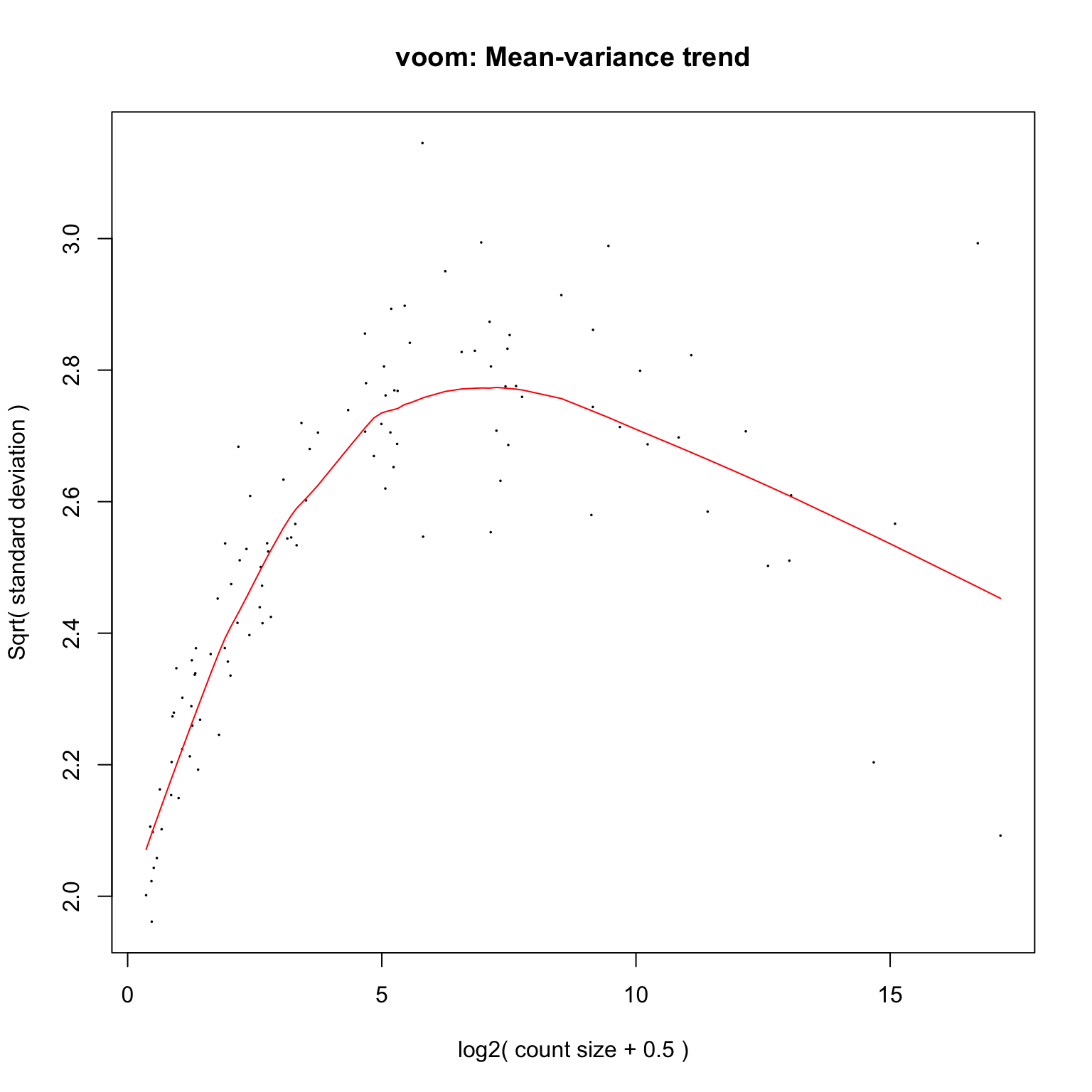
fit <- lmFit(y, mm)                                   #fit lm with limma
fit <- eBayes(fit)
head(coef(fit))
## (Intercept) groupKerala
## Prevotella_copri 16.1383696 -4.99436530
## Eubacterium_rectale 11.9161328 -0.08294369
## Butyrivibrio_crossotus -0.2110634 -0.08650380
## Prevotella_stercorea 6.8200020 -6.22106379
## Faecalibacterium_prausnitzii 13.6093282 1.00607350
## Subdoligranulum_unclassified 10.9786786 1.16771790limma_res_df <- data.frame(topTable(fit, coef = "groupKerala", number = Inf)) #extract results
fdr_limma <- limma_res_df %>%
dplyr::filter(adj.P.Val < 0.05) %>%
rownames_to_column(var = "Species")
dim(fdr_limma)## [1] 15 7head(fdr_limma)## Species logFC AveExpr t P.Value
## 1 Megasphaera_unclassified -8.974360 6.4247739 -5.575994 1.059729e-07
## 2 Bacteroides_coprocola -5.124762 -0.8291721 -4.484538 1.409614e-05
## 3 Prevotella_stercorea -6.221064 3.2149583 -3.867134 1.613340e-04
## 4 Lactobacillus_ruminis -5.711738 3.7967638 -3.833832 1.826516e-04
## 5 Ruminococcus_obeum 4.659230 2.7788048 3.737572 2.603217e-04
## 6 Mitsuokella_unclassified -5.237836 0.7101123 -3.732304 2.653693e-04
## adj.P.Val B
## 1 1.155105e-05 6.9755057
## 2 7.682395e-04 2.8793949
## 3 4.820876e-03 0.6994391
## 4 4.820876e-03 0.5749799
## 5 4.820876e-03 0.2933741
## 6 4.820876e-03 0.2931618ggplot(fdr_limma, aes(x = Species, y = logFC, color = Species)) +
geom_point(size = 4) +
labs(y = "\nLog2 Fold-Change for ACVD vs. Controls", x = "") +
theme(axis.text.x = element_text(color = "black", size = 12),
axis.text.y = element_text(color = "black", size = 12),
axis.title.y = element_text(size = 14),
axis.title.x = element_text(size = 14),
legend.text = element_text(size = 12),
legend.title = element_text(size = 12),
legend.position = "none") +
coord_flip() +
geom_hline(yintercept = 0, linetype="dotted")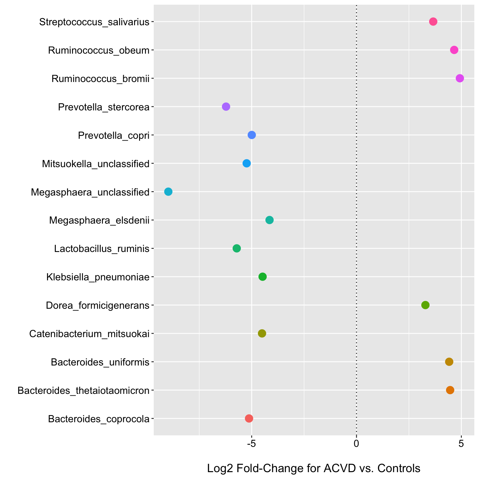
So we can see that limma-voom returned 15 species with an FDR corrected p-value < 0.05. Effect sizes may often be as or more informative than p-values alone for selecting DA features, but in these examples will will use the FDR p-value and a 0.05 threshold to retain features. The plot shows the log2 fold changes and could perhaps be improved by including estimates of the sampling variability etc.
DESeq2 with apeglm
dds <- DESeq(dds, test = "Wald", fitType = "local", sfType = "poscounts")## estimating size factors## estimating dispersions## gene-wise dispersion estimates## mean-dispersion relationship## final dispersion estimates## fitting model and testing## -- replacing outliers and refitting for 65 genes
## -- DESeq argument 'minReplicatesForReplace' = 7
## -- original counts are preserved in counts(dds)## estimating dispersions## fitting model and testingplotDispEsts(dds)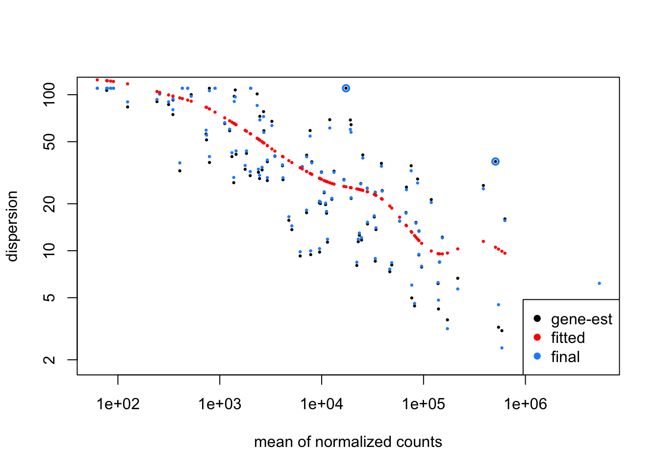
res <- lfcShrink(dds, coef=2, type="apeglm") ## using 'apeglm' for LFC shrinkage. If used in published research, please cite:
## Zhu, A., Ibrahim, J.G., Love, M.I. (2018) Heavy-tailed prior distributions for
## sequence count data: removing the noise and preserving large differences.
## Bioinformatics. https://doi.org/10.1093/bioinformatics/bty895plotMA(dds)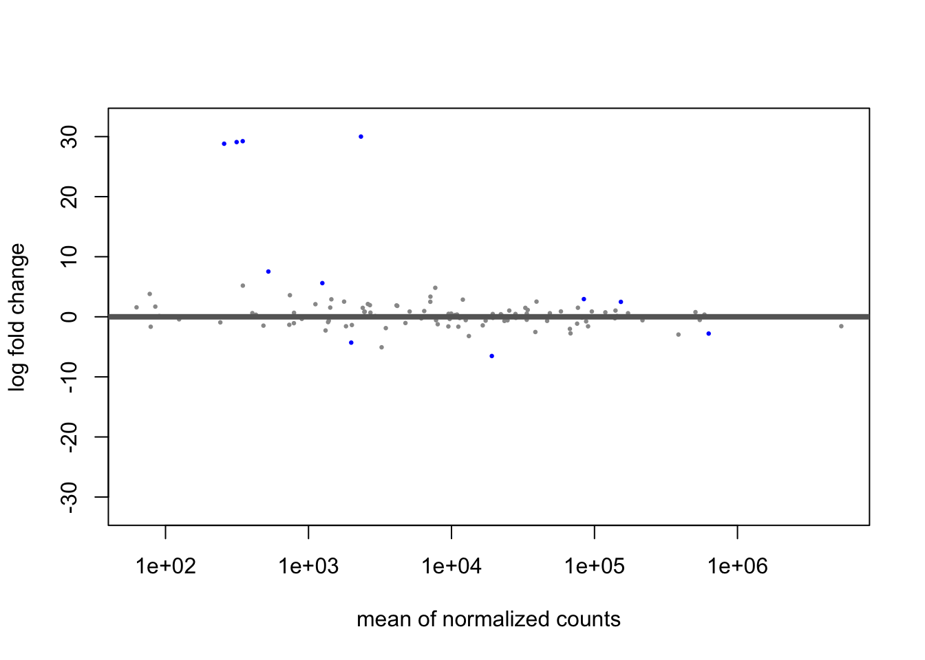
deseq_res_df <- data.frame(res) %>%
  rownames_to_column(var = "Species") %>%
  dplyr::arrange(padj)

fdr_deseq <- deseq_res_df %>%
    dplyr::filter(padj < 0.05)

dim(fdr_deseq)
## [1] 5 6head(fdr_deseq)## Species baseMean log2FoldChange lfcSE pvalue
## 1 Bacteroides_massiliensis 2326.9291 0.1667126 0.9692252 9.311151e-32
## 2 Clostridium_symbiosum 346.6204 0.5656621 1.2730261 4.669930e-32
## 3 Clostridium_hathewayi 314.3198 0.4874255 1.2012990 1.764584e-28
## 4 Parabacteroides_goldsteinii 256.9873 0.2564174 1.0225083 5.847951e-25
## 5 Bacteroides_coprocola 19141.8394 -0.7224703 1.3784468 2.200809e-03
## padj
## 1 4.934910e-30
## 2 4.934910e-30
## 3 6.234864e-27
## 4 1.549707e-23
## 5 4.665715e-02ggplot(fdr_deseq, aes(x = Species, y = log2FoldChange, color = Species)) +
geom_point(size = 4) +
labs(y = "\nLog2 Fold-Change for ACVD vs. Controls", x = "") +
theme(axis.text.x = element_text(color = "black", size = 12),
axis.text.y = element_text(color = "black", size = 12),
axis.title.y = element_text(size = 14),
axis.title.x = element_text(size = 14),
legend.text = element_text(size = 12),
legend.title = element_text(size = 12),
legend.position = "none") +
coord_flip() +
geom_hline(yintercept = 0, linetype="dotted")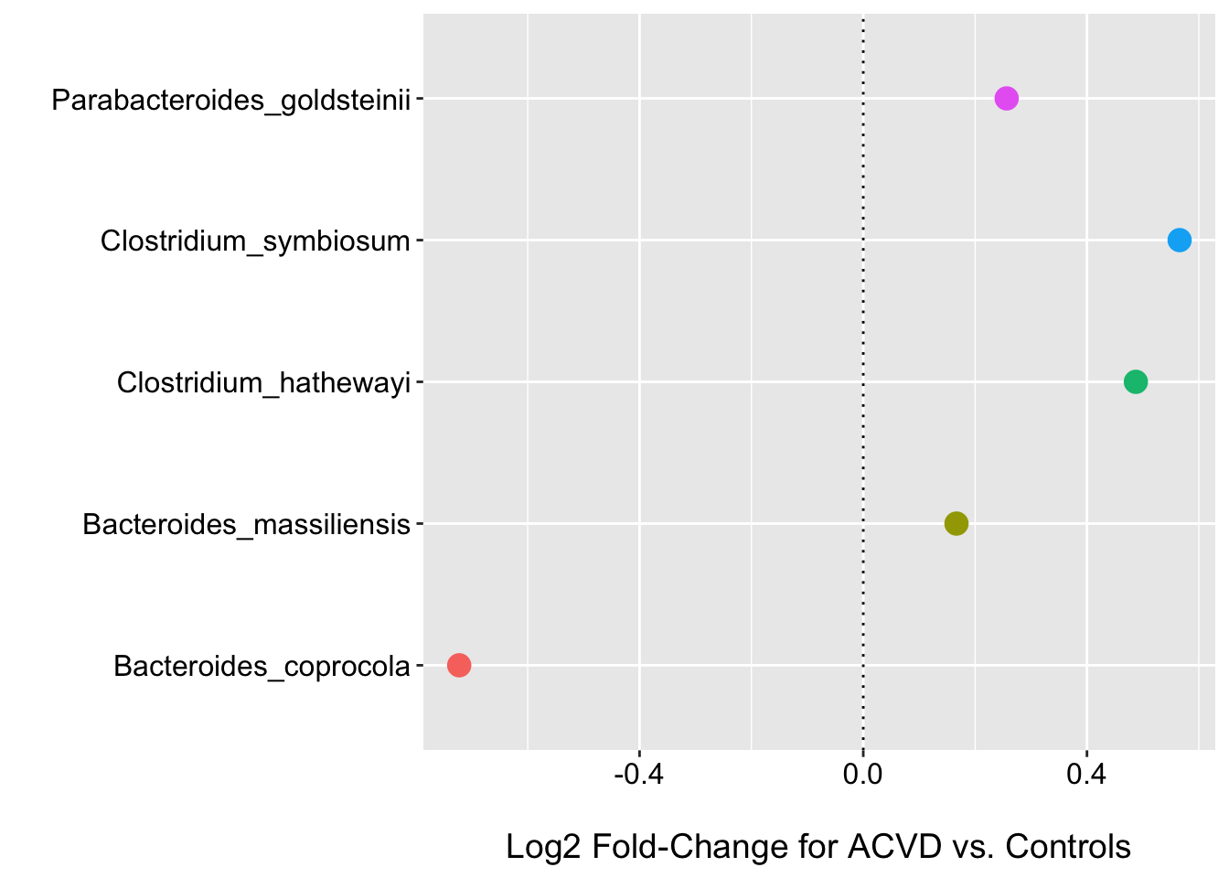
So we can see that DESeq2 returned 5 species with an FDR corrected p-value < 0.05. Here I show the log2 fold change plot as well. I will hold off on this for the rest of the methods, but similar plots can be generated based on the coefficient values etc. Take a look at the corncob tutorial for some examples of the different types of tests that can be performed.
Corncob
corn_da <- differentialTest(formula = ~ location,
                            phi.formula = ~ 1,
                            formula_null = ~ 1,
                            phi.formula_null = ~ 1,
                            data = ps,
                            test = "Wald", boot = FALSE,
                            fdr_cutoff = 0.05)

fdr_corncob <- corn_da$significant_taxa
dim(data.frame(fdr_corncob))
## [1] 28 1head(sort(corn_da$p_fdr)) ## Megasphaera_unclassified Ruminococcus_obeum
## 1.576463e-06 1.041461e-04
## Prevotella_stercorea Bacteroides_thetaiotaomicron
## 3.697782e-04 3.965007e-04
## Bacteroides_uniformis Lactobacillus_ruminis
## 4.262191e-04 5.608007e-04Corncob called 28 as DA. Here we are just testing the abundance. It might also be informative to include tests for differences in the dispersion.
MaAsLin 2
mas_1 <- Maaslin2(
  input_data = data.frame(otu_table(ps)),
  input_metadata = data.frame(sample_data(ps)),
  output = "/Users/olljt2/desktop/Maaslin2_default_output",
  min_abundance = 0.0,
  min_prevalence = 0.0,
  normalization = "TSS",
  transform = "LOG",
  analysis_method = "LM",
  max_significance = 0.05,
  fixed_effects = "location",
  correction = "BH",
  standardize = FALSE,
  cores = 1)
mas_res_df <- mas_1$results
fdr_mas <- mas_res_df %>%
dplyr::filter(qval < 0.05)
dim(fdr_mas)## [1] 27 10head(fdr_mas)## feature metadata value coef
## locationKerala32 Megasphaera_unclassified location Kerala -0.7713398
## locationKerala29 Ruminococcus_obeum location Kerala 0.6891505
## locationKerala14 Ruminococcus_bromii location Kerala 0.8985006
## locationKerala28 Bacteroides_thetaiotaomicron location Kerala 0.8813854
## locationKerala70 Streptococcus_salivarius location Kerala 0.5409692
## locationKerala3 Prevotella_stercorea location Kerala -1.0280049
## stderr pval name qval N
## locationKerala32 0.1583627 3.828477e-06 locationKerala 0.000417304 110
## locationKerala29 0.1577677 2.887477e-05 locationKerala 0.001573675 110
## locationKerala14 0.2122802 4.865394e-05 locationKerala 0.001767760 110
## locationKerala28 0.2271755 1.801616e-04 locationKerala 0.004347755 110
## locationKerala70 0.1404570 1.994383e-04 locationKerala 0.004347755 110
## locationKerala3 0.2774162 3.343767e-04 locationKerala 0.005206723 110
## N.not.zero
## locationKerala32 0
## locationKerala29 0
## locationKerala14 0
## locationKerala28 0
## locationKerala70 0
## locationKerala3 0MaAsLin 2 called 27 species as DA. Here we run the workflow under the default settings as the authors (surprisingly to me) found them to perform best across a range of scenarios in a recent paper. However, MaAsLin 2 allows for a wide range of transformations and models to be fit and I use it often to quickly fit different models to see how the choices impact the results. It can also accommodate random effects for some model selections.
ANCOM-BC
ancom_da <- ancombc(phyloseq = ps, formula = "location",
              p_adj_method = "fdr", zero_cut = 0.90, lib_cut = 1000,
              group = "location", struc_zero = TRUE, neg_lb = TRUE, tol = 1e-5,
              max_iter = 100, conserve = TRUE, alpha = 0.05, global = FALSE)

ancom_res_df <- data.frame(
  Species = row.names(ancom_da$res$beta),
  beta = unlist(ancom_da$res$beta),
  se = unlist(ancom_da$res$se),
  W = unlist(ancom_da$res$W),
  p_val = unlist(ancom_da$res$p_val),
  q_val = unlist(ancom_da$res$q_val),
  diff_abn = unlist(ancom_da$res$diff_abn))

fdr_ancom <- ancom_res_df %>%
  dplyr::filter(q_val < 0.05)

dim(fdr_ancom)
## [1] 15 7head(fdr_ancom)## Species beta se W
## locationKerala4 Prevotella_stercorea -4.414224 1.1839905 -3.728259
## locationKerala9 Mitsuokella_unclassified -3.467118 1.0176606 -3.406950
## locationKerala15 Ruminococcus_bromii 3.682311 1.0497644 3.507750
## locationKerala18 Lactobacillus_ruminis -3.608518 1.0441049 -3.456087
## locationKerala22 Catenibacterium_mitsuokai -3.055131 0.9621105 -3.175447
## locationKerala29 Bacteroides_thetaiotaomicron 3.143050 0.8682526 3.619973
## p_val q_val locationKerala
## locationKerala4 0.0001928069 0.006229387 TRUE
## locationKerala9 0.0006569326 0.007160566 TRUE
## locationKerala15 0.0004519128 0.007029239 TRUE
## locationKerala18 0.0005480782 0.007029239 TRUE
## locationKerala22 0.0014960575 0.013589189 TRUE
## locationKerala29 0.0002946343 0.006423028 TRUEThe new and improved ANCOM-BC called 15 species as DA. I have not yet seen external validation of the performance of this model, but look forward to how it might perform in head-to-head comparisons on diverse sets of simulated data.
Assessing overlap across approaches
Reduce(intersect, list(fdr_limma$Species, fdr_deseq$Species, fdr_corncob, fdr_mas$feature, fdr_ancom$Species)) #67 species## [1] "Bacteroides_coprocola"da_venn <- venn.diagram(
x = list(fdr_limma$Species, fdr_deseq$Species, fdr_corncob, fdr_mas$feature, fdr_ancom$Species),
category.names = c("Limma-Voom" , "DESeq2", "corncob", "MaAsLin2", "ANCOM-BC"),
filename = NULL,
fill = c("#8DD3C7", "#FFFFB3", "#BEBADA", "#FB8072", "#80B1D3"),
margin = 0.1)
grid::grid.newpage()
grid::grid.draw(da_venn) 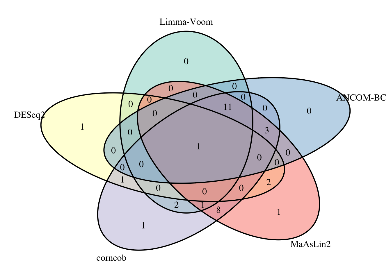
So only one species, Bacteroides coprocola, has a FDR p-value < 0.05 across all five methods. This might be a good place to start when considering which taxa might be changing most in relative abundance between conditions. You may also want to consider the effect size (i.e., the size of the fold change or coefficient) as well. It would also be reasonable to look at those taxa that were called as DA by multiple methods as well…and to perhaps dig into some of the taxa more deeply to try and understand if there are clear reasons for discrepancies between modeling approaches (i.e., excessive sparsity, etc.). For example, the 11 taxa called DA by all methods expect DESeq2 might be the next set of interest.
Of course, you will get different degrees of overlap when fitting these models to different datasets, but I hope this gives you a good start on how to consider fitting multiple models to identify potentially differentially abundant features.
Session Info
sessionInfo()## R version 4.0.4 (2021-02-15)
## Platform: x86_64-apple-darwin17.0 (64-bit)
## Running under: macOS Catalina 10.15.7
##
## Matrix products: default
## BLAS: /Library/Frameworks/R.framework/Versions/4.0/Resources/lib/libRblas.dylib
## LAPACK: /Library/Frameworks/R.framework/Versions/4.0/Resources/lib/libRlapack.dylib
##
## locale:
## [1] en_US.UTF-8/en_US.UTF-8/en_US.UTF-8/C/en_US.UTF-8/en_US.UTF-8
##
## attached base packages:
## [1] grid stats4 parallel stats graphics grDevices utils
## [8] datasets methods base
##
## other attached packages:
## [1] VennDiagram_1.6.20 futile.logger_1.4.3
## [3] Maaslin2_1.2.0 ANCOMBC_1.0.3
## [5] corncob_0.1.0 apeglm_1.10.0
## [7] DESeq2_1.28.1 SummarizedExperiment_1.18.2
## [9] DelayedArray_0.14.1 matrixStats_0.57.0
## [11] GenomicRanges_1.40.0 GenomeInfoDb_1.24.2
## [13] IRanges_2.22.2 S4Vectors_0.26.1
## [15] DEFormats_1.18.0 edgeR_3.30.3
## [17] limma_3.44.3 phyloseq_1.32.0
## [19] forcats_0.5.0 stringr_1.4.0
## [21] purrr_0.3.4 readr_1.3.1
## [23] tidyr_1.1.2 tibble_3.0.3
## [25] ggplot2_3.3.2 tidyverse_1.3.0
## [27] curatedMetagenomicData_1.18.2 ExperimentHub_1.14.2
## [29] dplyr_1.0.2 Biobase_2.48.0
## [31] AnnotationHub_2.20.2 BiocFileCache_1.12.1
## [33] dbplyr_1.4.4 BiocGenerics_0.34.0
##
## loaded via a namespace (and not attached):
## [1] ROI.plugin.lpsolve_1.0-0 tidyselect_1.1.0
## [3] RSQLite_2.2.0 AnnotationDbi_1.50.3
## [5] BiocParallel_1.22.0 Rtsne_0.15
## [7] munsell_0.5.0 codetools_0.2-18
## [9] withr_2.2.0 colorspace_1.4-1
## [11] lpSolveAPI_5.5.2.0-17.7 knitr_1.30
## [13] rstudioapi_0.11 robustbase_0.93-6
## [15] gbRd_0.4-11 Rdpack_2.0
## [17] labeling_0.3 optparse_1.6.6
## [19] slam_0.1-48 bbmle_1.0.23.1
## [21] GenomeInfoDbData_1.2.3 lpsymphony_1.16.0
## [23] bit64_4.0.5 farver_2.0.3
## [25] rhdf5_2.32.2 coda_0.19-4
## [27] vctrs_0.3.4 generics_0.0.2
## [29] lambda.r_1.2.4 xfun_0.19
## [31] R6_2.5.0 VGAM_1.1-4
## [33] locfit_1.5-9.4 bitops_1.0-6
## [35] microbiome_1.10.0 assertthat_0.2.1
## [37] promises_1.1.1 scales_1.1.1
## [39] gtable_0.3.0 rlang_0.4.8
## [41] genefilter_1.70.0 splines_4.0.4
## [43] trust_0.1-8 broom_0.7.0
## [45] checkmate_2.0.0 BiocManager_1.30.10
## [47] yaml_2.2.1 reshape2_1.4.4
## [49] modelr_0.1.8 backports_1.1.9
## [51] httpuv_1.5.4 tools_4.0.4
## [53] bookdown_0.21 logging_0.10-108
## [55] ellipsis_0.3.1 biomformat_1.16.0
## [57] RColorBrewer_1.1-2 hash_2.2.6.1
## [59] Rcpp_1.0.5 plyr_1.8.6
## [61] zlibbioc_1.34.0 RCurl_1.98-1.2
## [63] pbapply_1.4-3 ROI_1.0-0
## [65] haven_2.3.1 cluster_2.1.0
## [67] fs_1.5.0 magrittr_2.0.1
## [69] data.table_1.13.0 futile.options_1.0.1
## [71] blogdown_0.21.45 reprex_0.3.0
## [73] mvtnorm_1.1-1 hms_0.5.3
## [75] mime_0.9 evaluate_0.14
## [77] xtable_1.8-4 XML_3.99-0.5
## [79] emdbook_1.3.12 readxl_1.3.1
## [81] compiler_4.0.4 bdsmatrix_1.3-4
## [83] crayon_1.3.4 htmltools_0.5.0
## [85] mgcv_1.8-33 pcaPP_1.9-73
## [87] later_1.1.0.1 geneplotter_1.66.0
## [89] lubridate_1.7.9 DBI_1.1.0
## [91] formatR_1.7 biglm_0.9-2
## [93] MASS_7.3-53 rappdirs_0.3.1
## [95] Matrix_1.3-2 ade4_1.7-15
## [97] getopt_1.20.3 permute_0.9-5
## [99] cli_2.0.2 rbibutils_1.3
## [101] igraph_1.2.5 pkgconfig_2.0.3
## [103] registry_0.5-1 numDeriv_2016.8-1.1
## [105] xml2_1.3.2 foreach_1.5.0
## [107] annotate_1.66.0 multtest_2.44.0
## [109] XVector_0.28.0 rvest_0.3.6
## [111] detectseparation_0.1 digest_0.6.27
## [113] vegan_2.5-6 Biostrings_2.56.0
## [115] rmarkdown_2.5 cellranger_1.1.0
## [117] curl_4.3 shiny_1.5.0
## [119] nloptr_1.2.2.2 lifecycle_0.2.0
## [121] nlme_3.1-152 jsonlite_1.7.1
## [123] Rhdf5lib_1.10.1 fansi_0.4.1
## [125] pillar_1.4.6 lattice_0.20-41
## [127] fastmap_1.0.1 httr_1.4.2
## [129] DEoptimR_1.0-8 survival_3.2-7
## [131] interactiveDisplayBase_1.26.3 glue_1.4.2
## [133] iterators_1.0.12 BiocVersion_3.11.1
## [135] bit_4.0.4 stringi_1.5.3
## [137] blob_1.2.1 memoise_1.1.0
## [139] ape_5.4-1