Differential Feature Abundance Meta-Analysis
In a previous post, I highlighted some difficulties one faces with differential abundance (DA) testing when trying to identify those features (i.e., OTUs/ASVs, species, pathways, etc.) that “differ the most” according to some condition of interest. I examined the use of bootstrap ranking to assess the uncertainty in rankings when we have access to only a single study. In this post, I highlight how we can combine the results of multiple studies to obtain a pooled/summary estimate for a given feature when we have access to the primary data. While obtaining such data can often be difficult, one sometimes gets lucky given the increasing number of publicly available datasets.
Individual participant data meta-analysis (IPDMA) can be undertaken when one has access to the actual data for each study. Riley, Tierney & Stewart have an excellent textbook, materials, workshops, etc. on the topic on their website that I highly recommend. When we do not have access to the primary data, pooled/summary estimates can still be obtained if we can extract the required information (i.e., effect sizes and standard errors) from published studies (often this information is provided as a supplemental table). Of course in the latter case, we do not have the ability to standardize approaches (i.e., bioinformatic processing, variable harmonization, covariate adjustment, etc.) as we would when conducting an IPDMA.
In this post, I provide an example of how one can conduct a differential feature abundance meta-analysis. I use the curatedMetagenomicData package to access multiple studies examining differences in the stool microbiome of patients with colorectal cancer (CRC) when compared to otherwise healthy controls. There is not data on all relevant factors one might wish to adjust for to limit confounding bias (not sure I even have a good idea of what a sufficient adjustment set might look like), but these data were processed in a uniform fashion (all taxonomic profiles classified via MetaPhlAn3) and collected information on the condition of interest. So at a minimum we have a great dataset for a didactic example.
I will also look at the extent to which the results of a single large study align with the pooled estimates, since often, one does not have access to additional studies and published reports are based on the results of single (often underpowered) study. While I see the goals of meta-analysis and validation studies as being different, synthesizing the results of studies conducted in diverse cohorts can be informative in understanding variability in feature rankings (i.e, how do the results compare across studies, which features have the most “consistent” effects, etc.). In a future posts, I hope to use some simulated and real data sets to highlight the extent to which we might be able to drive down false positive results by including a validation cohort in our study design and what reasonable sample size requirements might actually be for differential abundance testing.
Load libraries
library(curatedMetagenomicData); packageVersion("curatedMetagenomicData") ## [1] '3.0.10'library(tidyverse); packageVersion("tidyverse") ## [1] '1.3.1'library(phyloseq); packageVersion("phyloseq") ## [1] '1.36.0'library(Maaslin2); packageVersion("Maaslin2") ## [1] '1.6.0'library(metafor); packageVersion("metafor") ## [1] '3.0.2'library(broom); packageVersion("broom") ## [1] '0.7.9'Identify CRC studies
First, we need to identify those studies that have data on both CRC cases and controls in the curatedMetagenomicData package. The sampleMetadata object is fantastic and makes such a search quite accessible. Here is a link to the curatedMetagenomicData package tutorial that explains in greater detail how to access data available through the package.
Basically, the code chunk below just runs a text search for studies with CRC in the disease field and retains those participant sample IDs where they provided a stool sample and were enrolled in a study containing both CRC cases and controls. This clearly looks much “cleaner” than the first time I ran this search and had to figure out what terms to use etc. This always takes me a little trial and error since there is a ton of information in the sampleMetadata object.
meta_df <- curatedMetagenomicData::sampleMetadata

crc_studies <- meta_df %>%
  dplyr::filter(grepl("CRC", disease)) %>%
  dplyr::distinct(study_name)
keep_studies <- crc_studies$study_name

crc_df <- meta_df %>%
  dplyr::filter(study_name %in% keep_studies) %>%
  dplyr::filter(study_condition %in% c("CRC", "control")) %>%
  dplyr::filter(body_site == "stool")

crc_df <- crc_df %>%
  dplyr::mutate(case_status = ifelse(str_detect(disease, "CRC"), "CRC",
                                     ifelse(disease == "healthy", "Control", "Other"))) %>%
  dplyr::filter(case_status != "Other")

mydata <- crc_df %>%
  dplyr::select(study_name, sample_id, subject_id, body_site, disease, age, gender,
BMI, country, sequencing_platform, DNA_extraction_kit)head(mydata)## study_name sample_id subject_id body_site disease age
## 1 FengQ_2015 SID31004 SID31004 stool CRC;fatty_liver;hypertension 64
## 2 FengQ_2015 SID31021 SID31021 stool healthy 60
## 3 FengQ_2015 SID31159 SID31159 stool CRC 73
## 4 FengQ_2015 SID31188 SID31188 stool CRC;fatty_liver;hypertension 65
## 5 FengQ_2015 SID31223 SID31223 stool CRC 65
## 6 FengQ_2015 SID31237 SID31237 stool CRC;fatty_liver;hypertension 67
## gender BMI country sequencing_platform DNA_extraction_kit
## 1 male 29.35 AUT IlluminaHiSeq MoBio
## 2 female 22.10 AUT IlluminaHiSeq MoBio
## 3 male 17.99 AUT IlluminaHiSeq MoBio
## 4 male 28.03 AUT IlluminaHiSeq MoBio
## 5 female 23.31 AUT IlluminaHiSeq MoBio
## 6 male 29.40 AUT IlluminaHiSeq MoBiomydata %>%
count(study_name)## study_name n
## 1 FengQ_2015 62
## 2 GuptaA_2019 60
## 3 HanniganGD_2017 55
## 4 ThomasAM_2018a 43
## 5 ThomasAM_2018b 60
## 6 ThomasAM_2019_c 80
## 7 VogtmannE_2016 104
## 8 WirbelJ_2018 125
## 9 YachidaS_2019 504
## 10 YuJ_2015 112
## 11 ZellerG_2014 114rm(list= ls()[!(ls() %in% c("mydata"))])We end up with 11 studies meeting these criteria and a fairly large number of samples (> 1300).
Download curated data
The returnSamples function allows us to pull down the processed microbiome data. Here I just pass the set of IDs I want to the function and request the taxonomic abundances as counts (as opposed to relative abundance as proportions).
Then I convert the data into a single phyloseq object. One could perform the subsequent analysis using the SummarizedExperiment object if preferred. I am just more comfortable working with phyloseq objects.
keep_id <- mydata$sample_id

crc_se_sp <- sampleMetadata %>%
  dplyr::filter(sample_id %in% keep_id) %>%
  curatedMetagenomicData::returnSamples("relative_abundance", counts = TRUE)

crc_sp_df <- as.data.frame(as.matrix(assay(crc_se_sp)))

crc_sp_df <- crc_sp_df %>%
  rownames_to_column(var = "Species")

otu_tab <- crc_sp_df %>%
  tidyr::separate(Species, into = c("Kingdom", "Phylum", "Class", "Order", "Family", "Genus", "Species"), sep = "\\|") %>%
  dplyr::select(-Kingdom, -Phylum, -Class, -Order, -Family, -Genus) %>%
  dplyr::mutate(Species = gsub("s__", "", Species)) %>%
  tibble::column_to_rownames(var = "Species")

tax_tab <- crc_sp_df %>%
  dplyr::select(Species) %>%
  tidyr::separate(Species, into = c("Kingdom", "Phylum", "Class", "Order", "Family", "Genus", "Species"), sep = "\\|") %>%
  dplyr::mutate(Kingdom = gsub("k__", "", Kingdom),
                Phylum = gsub("p__", "", Phylum),
                Class = gsub("c__", "", Class),
                Order = gsub("o__", "", Order),
                Family = gsub("f__", "", Family),
                Genus = gsub("g__", "", Genus),
                Species = gsub("s__", "", Species)) %>%
  dplyr::mutate(spec_row = Species) %>%
  tibble::column_to_rownames(var = "spec_row")

meta_df <- mydata %>%
  tibble::column_to_rownames(var = "sample_id")
(ps <- phyloseq(sample_data(meta_df),
otu_table(otu_tab, taxa_are_rows = TRUE),
tax_table(as.matrix(tax_tab))))## phyloseq-class experiment-level object
## otu_table() OTU Table: [ 934 taxa and 1319 samples ]
## sample_data() Sample Data: [ 1319 samples by 10 sample variables ]
## tax_table() Taxonomy Table: [ 934 taxa by 7 taxonomic ranks ]rm(list= ls()[!(ls() %in% c("ps"))])We can see that we now have a phyloseq object containing 934 taxa on 1319 samples with information on 7 taxonomic ranks and 10 sample variables. This is the information we need to conduct the meta-analysis.
Prepare data for DA testing
These code chunks clean up the metadata a bit, remove samples with low read counts, and remove taxa seen at less than 0.0001% relative abundance.
mydata <- data.frame(sample_data(ps)) %>%
  dplyr::select(-subject_id, -body_site, -DNA_extraction_kit) %>%
  na.omit(.) %>%
  dplyr::mutate(case_status = ifelse(str_detect(disease, "CRC"), "CRC",
                                     ifelse(disease == "healthy", "Control", "Other"))) %>%
  dplyr::filter(case_status != "Other") %>%
  dplyr::mutate(study_name = recode(study_name, ThomasAM_2019_c = "ThomasAM_2019"),
                study_name = factor(study_name,
                                    levels = c("ZellerG_2014", "FengQ_2015", "YuJ_2015",
                                               "VogtmannE_2016", "HanniganGD_2017", "ThomasAM_2018a",
                                               "ThomasAM_2018b", "WirbelJ_2018", "GuptaA_2019",
                                               "ThomasAM_2019", "YachidaS_2019")))

sample_data(ps)$study_name <- NULL

merge_meta <- mydata %>%
  dplyr::select(study_name, case_status)

ps <- merge_phyloseq(ps, sample_data(merge_meta))
(ps <- subset_samples(ps, !(is.na(case_status))))
## phyloseq-class experiment-level object
## otu_table() OTU Table: [ 934 taxa and 1304 samples ]
## sample_data() Sample Data: [ 1304 samples by 11 sample variables ]
## tax_table() Taxonomy Table: [ 934 taxa by 7 taxonomic ranks ]head(sort(sample_sums(ps))) ## MG100142 MG100163 SAMD00164886 MG100162 MG100164 MG100160
## 17146 330750 722269 2291325 2521950 2956655(ps <- subset_samples(ps, sample_sums(ps) > 10^6)) ## phyloseq-class experiment-level object
## otu_table() OTU Table: [ 934 taxa and 1301 samples ]
## sample_data() Sample Data: [ 1301 samples by 11 sample variables ]
## tax_table() Taxonomy Table: [ 934 taxa by 7 taxonomic ranks ]minTotRelAbun <- 1e-5
x <- taxa_sums(ps)
keepTaxa <- (x / sum(x)) > minTotRelAbun
(ps <- prune_taxa(keepTaxa, ps)) ## phyloseq-class experiment-level object
## otu_table() OTU Table: [ 462 taxa and 1301 samples ]
## sample_data() Sample Data: [ 1301 samples by 11 sample variables ]
## tax_table() Taxonomy Table: [ 462 taxa by 7 taxonomic ranks ]rm(x, keepTaxa, minTotRelAbun, mydata, merge_meta)Differential abundance estimates for Yachida et. al.
In a previous post, I presented results using the same workflow for the Yachida et. al. 2019 data alone.
Here we reproduce those results to see how how the findings from a single, large study agree with the pooled/summary estimates obtained across all studies.
We will perform the DA testing using the popular Maaslin2 package with the default settings (as recommended here). See my previous post for a few other workflows (among the list of many dozens of available) that could be used if interested.
ps_y <- subset_samples(ps, study_name == "YachidaS_2019")

m_y <- Maaslin2(
  input_data = data.frame(otu_table(ps_y)),
  input_metadata = data.frame(sample_data(ps_y)),
  output = "/Users/olljt2/desktop/maaslin2_output",
  min_abundance = 0.0,
  min_prevalence = 0.3,
  normalization = "TSS",
  transform = "LOG",
  analysis_method = "LM",
  fixed_effects = c("age", "gender", "BMI", "case_status"),
  correction = "BH",
  standardize = FALSE,
  cores = 1,
  plot_heatmap = FALSE,
  plot_scatter = FALSE)

mas_y_out <- m_y$results %>%
  dplyr::filter(metadata == "case_status") %>%
dplyr::select(-qval, -name, -metadata, -N, -N.not.zero)head(mas_y_out)## feature value coef stderr pval
## 1 Collinsella_aerofaciens CRC 1.7140080 0.4373069 0.0001011899
## 2 Roseburia_faecis CRC -1.7735569 0.4542806 0.0001076316
## 3 Holdemania_filiformis CRC 1.1320742 0.3153403 0.0003634875
## 4 Bacteroides_cellulosilyticus CRC 1.6529415 0.4741172 0.0005330389
## 5 Streptococcus_anginosus_group CRC 0.8565514 0.2613467 0.0011207718
## 6 Mogibacterium_diversum CRC 0.9207161 0.2961708 0.0019866209As before, we see that Collinsella aerofaciens has the lowest p-value and thus may be considered (depending on one’s criteria) among the most differentially abundant species. We also see Roseburia faecis, Holdemania filiformis, Bacteroides cellulosilyticus, Streptococcus anginosus, and Mogibacterium diversum among the “top hits”.
Meta-Analysis: Stage 1
In the next two sections, I show how one can conduct a two-stage meta-analysis for each species that is seen in at least three studies. In stage 1, we obtain the estimated coefficient values and standard errors for each species in each study. In stage 2, we pool the results to obtain a summary estimate.
To obtain the stage 1 estimates we:
- generate a phyloseq object for each study and combine them all in single a list object
- write a function to run the Maaslin2 workflow and return the results for each species as a data.frame
- apply the function to each ps object/study in the list
- combine the results as a data.frame
Here the estimate for case_status is of interest and we include age, gender, and BMI as model covariates. All other selections are set to the Maaslin2 defaults other than suppressing some of the output. I use only one core here since these models take only a few moments to run.
The first line of code below just cleans up the sample names so they do not cause us problems later on (best practice IMO is never to use leading numbers or to include special characters other than underscores in your sample names or they can/will cause you issues/headaches later on).
sample_names(ps) <- gsub("\\-", "_", sample_names(ps))

FengQ_2015 <- subset_samples(ps, study_name == "FengQ_2015")
GuptaA_2019 <- subset_samples(ps, study_name == "GuptaA_2019")
HanniganGD_2017 <- subset_samples(ps, study_name == "HanniganGD_2017")
ThomasAM_2018a <- subset_samples(ps, study_name == "ThomasAM_2018a")
ThomasAM_2018b <- subset_samples(ps, study_name == "ThomasAM_2018b")
ThomasAM_2019 <- subset_samples(ps, study_name == "ThomasAM_2019")
VogtmannE_2016 <- subset_samples(ps, study_name == "VogtmannE_2016")
WirbelJ_2018 <- subset_samples(ps, study_name == "WirbelJ_2018")
YachidaS_2019 <- subset_samples(ps, study_name == "YachidaS_2019")
YuJ_2015 <- subset_samples(ps, study_name == "YuJ_2015")
ZellerG_2014 <- subset_samples(ps, study_name == "ZellerG_2014")

ps_list <- list(FengQ_2015 = FengQ_2015,
                GuptaA_2019 = GuptaA_2019,
                HanniganGD_2017 = HanniganGD_2017,
                ThomasAM_2018a = ThomasAM_2018a,
                ThomasAM_2018b = ThomasAM_2018b,
                ThomasAM_2019 = ThomasAM_2019,
                VogtmannE_2016 = VogtmannE_2016,
                WirbelJ_2018 = WirbelJ_2018,
                YachidaS_2019 = YachidaS_2019,
                YuJ_2015 = YuJ_2015,
                ZellerG_2014 = ZellerG_2014)

ps_list
## $FengQ_2015
## phyloseq-class experiment-level object
## otu_table() OTU Table: [ 462 taxa and 62 samples ]
## sample_data() Sample Data: [ 62 samples by 11 sample variables ]
## tax_table() Taxonomy Table: [ 462 taxa by 7 taxonomic ranks ]
##
## $GuptaA_2019
## phyloseq-class experiment-level object
## otu_table() OTU Table: [ 462 taxa and 60 samples ]
## sample_data() Sample Data: [ 60 samples by 11 sample variables ]
## tax_table() Taxonomy Table: [ 462 taxa by 7 taxonomic ranks ]
##
## $HanniganGD_2017
## phyloseq-class experiment-level object
## otu_table() OTU Table: [ 462 taxa and 52 samples ]
## sample_data() Sample Data: [ 52 samples by 11 sample variables ]
## tax_table() Taxonomy Table: [ 462 taxa by 7 taxonomic ranks ]
##
## $ThomasAM_2018a
## phyloseq-class experiment-level object
## otu_table() OTU Table: [ 462 taxa and 40 samples ]
## sample_data() Sample Data: [ 40 samples by 11 sample variables ]
## tax_table() Taxonomy Table: [ 462 taxa by 7 taxonomic ranks ]
##
## $ThomasAM_2018b
## phyloseq-class experiment-level object
## otu_table() OTU Table: [ 462 taxa and 58 samples ]
## sample_data() Sample Data: [ 58 samples by 11 sample variables ]
## tax_table() Taxonomy Table: [ 462 taxa by 7 taxonomic ranks ]
##
## $ThomasAM_2019
## phyloseq-class experiment-level object
## otu_table() OTU Table: [ 462 taxa and 80 samples ]
## sample_data() Sample Data: [ 80 samples by 11 sample variables ]
## tax_table() Taxonomy Table: [ 462 taxa by 7 taxonomic ranks ]
##
## $VogtmannE_2016
## phyloseq-class experiment-level object
## otu_table() OTU Table: [ 462 taxa and 101 samples ]
## sample_data() Sample Data: [ 101 samples by 11 sample variables ]
## tax_table() Taxonomy Table: [ 462 taxa by 7 taxonomic ranks ]
##
## $WirbelJ_2018
## phyloseq-class experiment-level object
## otu_table() OTU Table: [ 462 taxa and 125 samples ]
## sample_data() Sample Data: [ 125 samples by 11 sample variables ]
## tax_table() Taxonomy Table: [ 462 taxa by 7 taxonomic ranks ]
##
## $YachidaS_2019
## phyloseq-class experiment-level object
## otu_table() OTU Table: [ 462 taxa and 502 samples ]
## sample_data() Sample Data: [ 502 samples by 11 sample variables ]
## tax_table() Taxonomy Table: [ 462 taxa by 7 taxonomic ranks ]
##
## $YuJ_2015
## phyloseq-class experiment-level object
## otu_table() OTU Table: [ 462 taxa and 111 samples ]
## sample_data() Sample Data: [ 111 samples by 11 sample variables ]
## tax_table() Taxonomy Table: [ 462 taxa by 7 taxonomic ranks ]
##
## $ZellerG_2014
## phyloseq-class experiment-level object
## otu_table() OTU Table: [ 462 taxa and 110 samples ]
## sample_data() Sample Data: [ 110 samples by 11 sample variables ]
## tax_table() Taxonomy Table: [ 462 taxa by 7 taxonomic ranks ]get_s1_coef <- function(ps_object){
m <- Maaslin2(
input_data = data.frame(otu_table(ps_object)),
input_metadata = data.frame(sample_data(ps_object)),
output = "/Users/olljt2/desktop/maaslin2_output",
min_abundance = 0.0,
min_prevalence = 0.3,
normalization = "TSS",
transform = "LOG",
analysis_method = "LM",
fixed_effects = c("age", "gender", "BMI", "case_status"),
correction = "BH",
standardize = FALSE,
cores = 1,
plot_heatmap = FALSE,
plot_scatter = FALSE)
mas_out <- m$results %>%
dplyr::filter(metadata == "case_status") %>%
dplyr::select(-qval, -name, -metadata, -N, -N.not.zero)
return(mas_out)
}
stage_1_res <- lapply(ps_list, get_s1_coef)
s1_res_df <- bind_rows(stage_1_res, .id = "column_label")print.data.frame(head(s1_res_df))## column_label feature value coef stderr
## 1 FengQ_2015 Escherichia_coli CRC 5.882174 1.3664527
## 2 FengQ_2015 Prevotella_copri CRC 6.079525 1.4439969
## 3 FengQ_2015 Eubacterium_sp_CAG_251 CRC -7.014662 1.8576141
## 4 FengQ_2015 Fusicatenibacter_saccharivorans CRC -1.800875 0.5530868
## 5 FengQ_2015 Coprococcus_comes CRC -3.200692 1.0025953
## 6 FengQ_2015 Alistipes_finegoldii CRC 3.949649 1.2227965
## pval
## 1 6.650347e-05
## 2 9.159924e-05
## 3 3.821179e-04
## 4 1.904298e-03
## 5 2.297237e-03
## 6 2.056689e-03Meta-Analysis: Stage 2
You can see from the rows printed above that we now have a data.frame that contains the effect size and SE for each species, in each study, that we need to generate the pooled/summary estimates.
In stage 2, we generate pooled estimates using the random-effects MA model fitted via restricted maximum likelihood provided in the metafor package. I only generate pooled estimates for species seen in at least 3 studies and use the Knapp and Hartung adjustment for the standard errors to help account for uncertainty in the estimate of the amount of (residual) heterogeneity.
I use a bit of tidyverse code with purr::map to iterate over nested data.frames, organize the results using broom, and calculate an FDR p-value for each species (should one consider it to be of use).
I also print the first few rows of the output data.frame so we can see the results. Often I will convert the Maaslin2 default output to the log2 scale for comparisons to other models [e.g., log2(exp(coef))]. However, here I just use the default output and refer to the log relative abundances as the “effect size” measure.
prev_taxa <- s1_res_df %>%
  dplyr::count(feature) %>%
  dplyr::filter(n > 2)

keep_taxa <- prev_taxa$feature

s1_res_filt_df <- s1_res_df %>%
  dplyr::filter(feature %in% keep_taxa)     #retain species seen in at least 3 studies for MA


s2_res_df <- s1_res_filt_df %>%
  dplyr::rename("study_name" = "column_label") %>%
  dplyr::select(-pval, -value) %>%
  tidyr::nest(data = c(study_name, coef, stderr)) %>%
  dplyr::mutate(model = map(data, ~rma(yi = coef, sei = stderr, data = ., method = "REML", knha = TRUE))) %>%
  dplyr::mutate(tidy_model = map(model, tidy, conf.int = TRUE, exponentiate = FALSE)) %>%
  select(-data, -model) %>%
  unnest(cols = c(tidy_model)) %>%
  dplyr::select(-type, -term) %>%
  dplyr::arrange(p.value) %>%
  dplyr::mutate(fdr_pval = p.adjust(p.value, method = "fdr"))

print.data.frame(head(s2_res_df))
## feature estimate std.error statistic p.value conf.low
## 1 Clostridium_symbiosum 2.0741083 0.3646613 5.687767 0.0007447156 1.2118215
## 2 Bacteroides_fragilis 1.6558011 0.3639436 4.549609 0.0013867145 0.8325034
## 3 Bilophila_wadsworthia 0.7938644 0.1691665 4.692799 0.0015558825 0.4037657
## 4 Eisenbergiella_tayi 1.6555579 0.2715053 6.097699 0.0017171969 0.9576312
## 5 Roseburia_intestinalis -1.4338628 0.3306763 -4.336152 0.0018880488 -2.1819046
## 6 Hungatella_hathewayi 1.6063510 0.3615452 4.443016 0.0021592643 0.7726263
## conf.high fdr_pval
## 1 2.936395 0.03871462
## 2 2.479099 0.03871462
## 3 1.183963 0.03871462
## 4 2.353485 0.03871462
## 5 -0.685821 0.03871462
## 6 2.440076 0.03871462Comparing Yachida to pooled estimates
Collinsella aerofaciens had the lowest p-value (low FDR p-value if calculated) and thus, by that metric, might be considered the “top hit”.
This code chunk lets us see how this species stacks up across studies.
ca_df <- s1_res_df %>%
  filter(feature == "Collinsella_aerofaciens")

(ca_res <- rma(yi = coef, sei = stderr, method = "REML", knha = TRUE, data = ca_df))
##
## Random-Effects Model (k = 11; tau^2 estimator: REML)
##
## tau^2 (estimated amount of total heterogeneity): 1.2185 (SE = 0.8904)
## tau (square root of estimated tau^2 value): 1.1038
## I^2 (total heterogeneity / total variability): 64.13%
## H^2 (total variability / sampling variability): 2.79
##
## Test for Heterogeneity:
## Q(df = 10) = 28.6296, p-val = 0.0014
##
## Model Results:
##
## estimate se tval df pval ci.lb ci.ub
## 0.2929 0.4237 0.6912 10 0.5051 -0.6511 1.2369
##
## ---
## Signif. codes: 0 '***' 0.001 '**' 0.01 '*' 0.05 '.' 0.1 ' ' 1forest(ca_res, addfit = TRUE, showweights = TRUE, header = TRUE,
slab = ca_df$column_label,
xlab = "Coef [95% CI]", mlab = "Random Effects Model:\nCollinsella aerofaciens")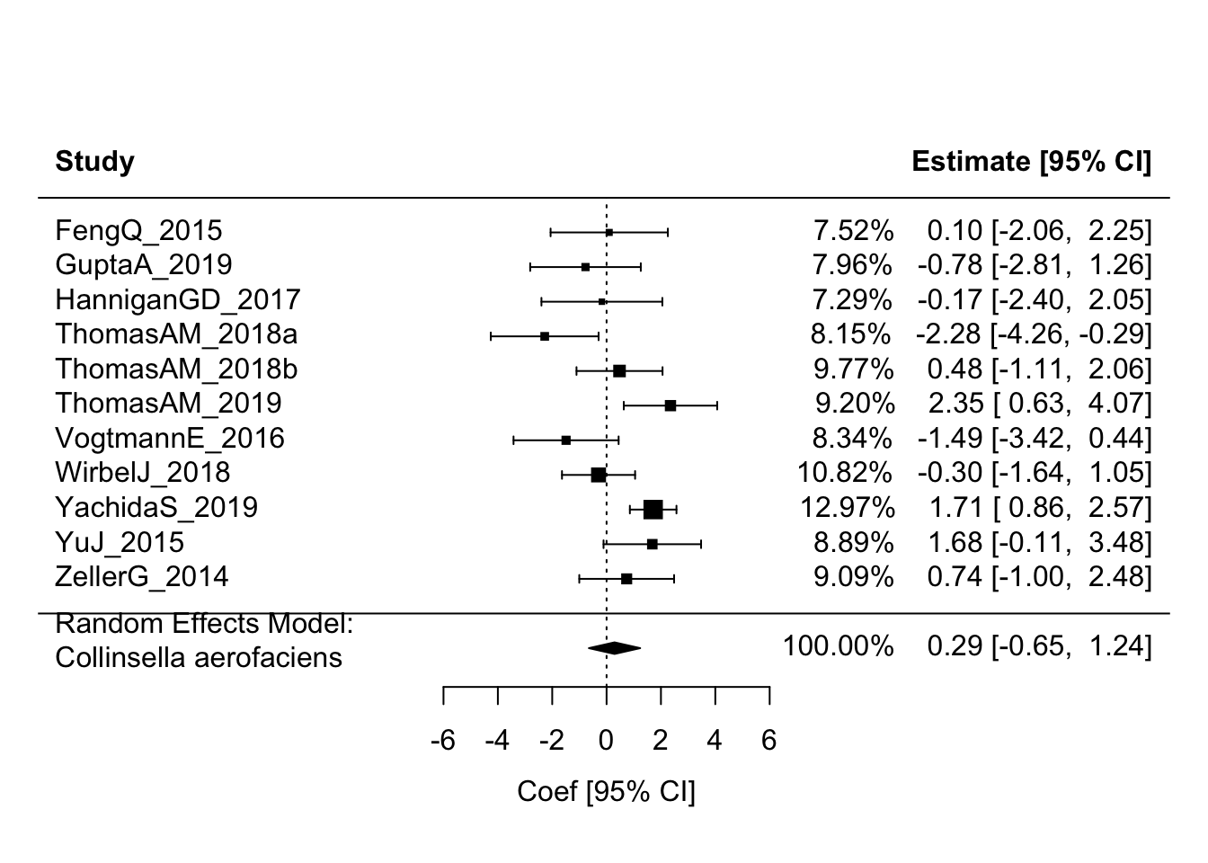
We see less impressive results in the pooled analysis for this particular species. This may not be entirety unexpected since, when we try to “pick winners” this way from a single study, we are by definition selecting the most extreme results without any attempt to account for the fact that the effect might be expected to regress back toward some less extreme value if we ran this same process again (or many times) in a new set of samples drawn from the same study population of interest. Of course here we have samples from diverse cohorts, so the attenuation may also reflect true differences in the correlation across these different “study populations”. I do not dig into that here.
Let’s look at the other top hits in the Yachida et. al. data.
my_taxa <- c("Collinsella_aerofaciens", "Roseburia_faecis", "Holdemania_filiformis",
             "Bacteroides_cellulosilyticus", "Streptococcus_anginosus_group", "Mogibacterium_diversum")

my_res <- s2_res_df %>%
  dplyr::filter(feature %in% my_taxa)

print.data.frame(head(my_res))
## feature estimate std.error statistic p.value
## 1 Streptococcus_anginosus_group 1.0697916 0.2147448 4.9816887 0.004169671
## 2 Mogibacterium_diversum 0.8322284 0.1786965 4.6572164 0.005545968
## 3 Holdemania_filiformis 0.6255553 0.3987170 1.5689208 0.160655175
## 4 Roseburia_faecis -1.0002745 0.6799560 -1.4710871 0.172021690
## 5 Bacteroides_cellulosilyticus 0.4047686 0.4269421 0.9480643 0.370851454
## 6 Collinsella_aerofaciens 0.2928582 0.4236712 0.6912392 0.505144955
## conf.low conf.high fdr_pval
## 1 0.5177726 1.6218107 0.04875308
## 2 0.3728744 1.2915825 0.05619914
## 3 -0.3172605 1.5683712 0.31307162
## 4 -2.5153109 0.5147619 0.32280613
## 5 -0.5797617 1.3892988 0.58112805
## 6 -0.6511401 1.2368565 0.67352661Streptococcus anginosus and Mogibacterium diversum still look like good candidates based on the pooled results. The other four less so. Let’s generate a forest plot for Streptococcus anginosus.
sa_df <- s1_res_df %>%
  filter(feature == "Streptococcus_anginosus_group")

(sa_res <- rma(yi = coef, sei = stderr, method = "REML", knha = TRUE, data = sa_df))
##
## Random-Effects Model (k = 6; tau^2 estimator: REML)
##
## tau^2 (estimated amount of total heterogeneity): 0.0144 (SE = 0.1866)
## tau (square root of estimated tau^2 value): 0.1199
## I^2 (total heterogeneity / total variability): 4.05%
## H^2 (total variability / sampling variability): 1.04
##
## Test for Heterogeneity:
## Q(df = 5) = 5.1779, p-val = 0.3946
##
## Model Results:
##
## estimate se tval df pval ci.lb ci.ub
## 1.0698 0.2147 4.9817 5 0.0042 0.5178 1.6218 **
##
## ---
## Signif. codes: 0 '***' 0.001 '**' 0.01 '*' 0.05 '.' 0.1 ' ' 1forest(sa_res, addfit = TRUE, showweights = TRUE, header = TRUE,
slab = sa_df$column_label,
xlab = "Coef [95% CI]", mlab = "Random Effects Model:\nStreptococcus anginosus")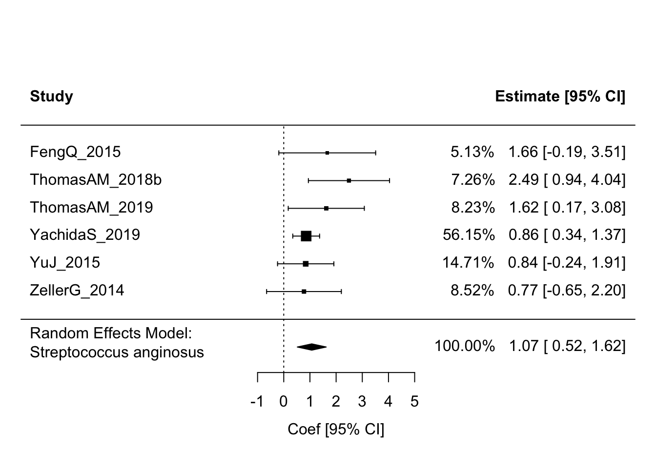
Here we see the summary estimate is dominated by the Yachida data (large sample size and low variance), but the effects are in the same direction across all studies providing additional support for perhaps a more “generalizable” association.
Species with low pooled FDR p-values
In this code chunk, I print the top taxa with the lowest FDR p-values based on the pooled estimates, plot the “top hits”, and generate a forest plot for Bacteroides fragilis.
print.data.frame(head(s2_res_df))## feature estimate std.error statistic p.value conf.low
## 1 Clostridium_symbiosum 2.0741083 0.3646613 5.687767 0.0007447156 1.2118215
## 2 Bacteroides_fragilis 1.6558011 0.3639436 4.549609 0.0013867145 0.8325034
## 3 Bilophila_wadsworthia 0.7938644 0.1691665 4.692799 0.0015558825 0.4037657
## 4 Eisenbergiella_tayi 1.6555579 0.2715053 6.097699 0.0017171969 0.9576312
## 5 Roseburia_intestinalis -1.4338628 0.3306763 -4.336152 0.0018880488 -2.1819046
## 6 Hungatella_hathewayi 1.6063510 0.3615452 4.443016 0.0021592643 0.7726263
## conf.high fdr_pval
## 1 2.936395 0.03871462
## 2 2.479099 0.03871462
## 3 1.183963 0.03871462
## 4 2.353485 0.03871462
## 5 -0.685821 0.03871462
## 6 2.440076 0.03871462my_plot <- s2_res_df %>%
dplyr::filter(fdr_pval < 0.1) %>%
mutate(high = ifelse(estimate > 0, "high", "low"),
feature = fct_reorder(feature, estimate))
ggplot(data = my_plot, aes(x = feature, y = estimate, fill = high)) +
geom_col(alpha = .8) +
labs(y = "\nEffect Size", x = "") +
theme(axis.text.x = element_text(color = "black", size = 8),
axis.text.y = element_text(color = "black", size = 8),
axis.title.y = element_text(size = 8),
axis.title.x = element_text(size = 10),
legend.text = element_text(size = 8),
legend.title = element_text(size = 8)) +
coord_flip() +
geom_hline(yintercept = 0, linetype="dotted") +
scale_fill_manual("legend", values = c("high" = "#00BFC4", "low" = "#F8766D")) +
theme(legend.position = "none")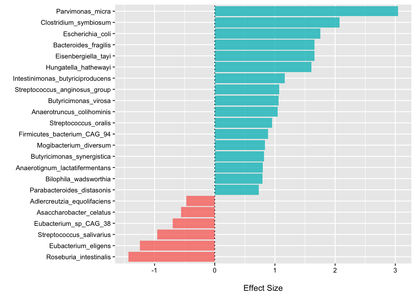
bf_df <- s1_res_df %>%
  filter(feature == "Bacteroides_fragilis")

(bf_res <- rma(yi = coef, sei = stderr, method = "REML", knha = TRUE, data = bf_df))
##
## Random-Effects Model (k = 10; tau^2 estimator: REML)
##
## tau^2 (estimated amount of total heterogeneity): 0.6474 (SE = 0.7253)
## tau (square root of estimated tau^2 value): 0.8046
## I^2 (total heterogeneity / total variability): 43.83%
## H^2 (total variability / sampling variability): 1.78
##
## Test for Heterogeneity:
## Q(df = 9) = 16.3556, p-val = 0.0598
##
## Model Results:
##
## estimate se tval df pval ci.lb ci.ub
## 1.6558 0.3639 4.5496 9 0.0014 0.8325 2.4791 **
##
## ---
## Signif. codes: 0 '***' 0.001 '**' 0.01 '*' 0.05 '.' 0.1 ' ' 1forest(bf_res, addfit = TRUE, showweights = TRUE, header = TRUE,
slab = bf_df$column_label,
xlab = "Coef [95% CI]", mlab = "Random Effects Model:\nBacteroides fragilis")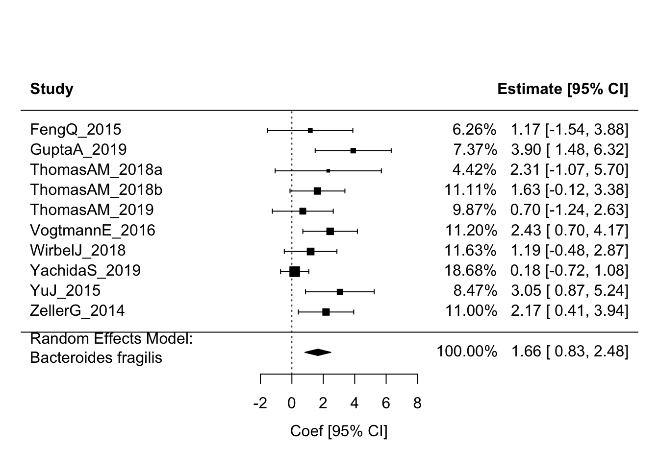
The main point of this post is that synthesizing the results of multiple studies may provide us with some additional insight into the potential variability in feature rankings that is missed when we have access to only a single study. As more and more results and datasets from microbiome studies are published, the opportunities to learn from the application of meta-analytic approaches is increased.
Session Info
sessionInfo()## R version 4.1.1 (2021-08-10)
## Platform: x86_64-apple-darwin17.0 (64-bit)
## Running under: macOS Catalina 10.15.7
##
## Matrix products: default
## BLAS: /Library/Frameworks/R.framework/Versions/4.1/Resources/lib/libRblas.0.dylib
## LAPACK: /Library/Frameworks/R.framework/Versions/4.1/Resources/lib/libRlapack.dylib
##
## locale:
## [1] en_US.UTF-8/en_US.UTF-8/en_US.UTF-8/C/en_US.UTF-8/en_US.UTF-8
##
## attached base packages:
## [1] parallel stats4 stats graphics grDevices utils datasets
## [8] methods base
##
## other attached packages:
## [1] broom_0.7.9 metafor_3.0-2
## [3] Matrix_1.3-4 Maaslin2_1.6.0
## [5] phyloseq_1.36.0 forcats_0.5.1
## [7] stringr_1.4.0 dplyr_1.0.7
## [9] purrr_0.3.4 readr_2.0.2
## [11] tidyr_1.1.4 tibble_3.1.5
## [13] ggplot2_3.3.5 tidyverse_1.3.1
## [15] curatedMetagenomicData_3.0.10 TreeSummarizedExperiment_2.0.3
## [17] Biostrings_2.60.2 XVector_0.32.0
## [19] SingleCellExperiment_1.14.1 SummarizedExperiment_1.22.0
## [21] Biobase_2.52.0 GenomicRanges_1.44.0
## [23] GenomeInfoDb_1.28.4 IRanges_2.26.0
## [25] S4Vectors_0.30.2 BiocGenerics_0.38.0
## [27] MatrixGenerics_1.4.3 matrixStats_0.61.0
##
## loaded via a namespace (and not attached):
## [1] readxl_1.3.1 backports_1.2.1
## [3] AnnotationHub_3.0.2 BiocFileCache_2.0.0
## [5] plyr_1.8.6 igraph_1.2.7
## [7] lazyeval_0.2.2 splines_4.1.1
## [9] BiocParallel_1.26.2 lpsymphony_1.20.0
## [11] digest_0.6.28 foreach_1.5.1
## [13] htmltools_0.5.2 fansi_0.5.0
## [15] magrittr_2.0.1 memoise_2.0.0
## [17] cluster_2.1.2 tzdb_0.1.2
## [19] modelr_0.1.8 colorspace_2.0-2
## [21] blob_1.2.2 rvest_1.0.2
## [23] rappdirs_0.3.3 haven_2.4.3
## [25] xfun_0.29 crayon_1.4.1
## [27] RCurl_1.98-1.5 jsonlite_1.7.2
## [29] biglm_0.9-2.1 hash_2.2.6.1
## [31] survival_3.2-11 iterators_1.0.13
## [33] ape_5.5 glue_1.4.2
## [35] gtable_0.3.0 zlibbioc_1.38.0
## [37] DelayedArray_0.18.0 Rhdf5lib_1.14.2
## [39] DEoptimR_1.0-9 scales_1.1.1
## [41] mvtnorm_1.1-3 DBI_1.1.1
## [43] Rcpp_1.0.7 xtable_1.8-4
## [45] tidytree_0.3.5 bit_4.0.4
## [47] getopt_1.20.3 httr_1.4.2
## [49] ellipsis_0.3.2 farver_2.1.0
## [51] pkgconfig_2.0.3 sass_0.4.0
## [53] dbplyr_2.1.1 utf8_1.2.2
## [55] labeling_0.4.2 tidyselect_1.1.1
## [57] rlang_0.4.12 reshape2_1.4.4
## [59] later_1.3.0 AnnotationDbi_1.54.1
## [61] munsell_0.5.0 BiocVersion_3.13.1
## [63] cellranger_1.1.0 tools_4.1.1
## [65] cachem_1.0.6 cli_3.1.0
## [67] generics_0.1.1 RSQLite_2.2.8
## [69] ExperimentHub_2.0.0 ade4_1.7-18
## [71] mathjaxr_1.4-0 evaluate_0.14
## [73] biomformat_1.20.0 fastmap_1.1.0
## [75] yaml_2.2.1 knitr_1.36
## [77] bit64_4.0.5 fs_1.5.0
## [79] robustbase_0.93-9 KEGGREST_1.32.0
## [81] pbapply_1.5-0 nlme_3.1-152
## [83] mime_0.12 xml2_1.3.2
## [85] compiler_4.1.1 rstudioapi_0.13
## [87] filelock_1.0.2 curl_4.3.2
## [89] png_0.1-7 interactiveDisplayBase_1.30.0
## [91] reprex_2.0.1 treeio_1.16.2
## [93] pcaPP_1.9-74 bslib_0.3.1
## [95] stringi_1.7.5 highr_0.9
## [97] blogdown_1.7 lattice_0.20-44
## [99] vegan_2.5-7 permute_0.9-5
## [101] multtest_2.48.0 vctrs_0.3.8
## [103] pillar_1.6.4 lifecycle_1.0.1
## [105] rhdf5filters_1.4.0 optparse_1.7.1
## [107] BiocManager_1.30.16 jquerylib_0.1.4
## [109] data.table_1.14.2 bitops_1.0-7
## [111] httpuv_1.6.3 R6_2.5.1
## [113] bookdown_0.24 promises_1.2.0.1
## [115] codetools_0.2-18 MASS_7.3-54
## [117] assertthat_0.2.1 rhdf5_2.36.0
## [119] withr_2.4.2 GenomeInfoDbData_1.2.6
## [121] mgcv_1.8-36 hms_1.1.1
## [123] grid_4.1.1 rmarkdown_2.11
## [125] logging_0.10-108 shiny_1.7.1
## [127] lubridate_1.8.0