Examining Coverage of CLR Regression
I was thinking recently about the performance of linear models for differential abundance testing in microbiome studies (see here for an example) despite the sparse, extremely non-normal, and compositional nature of mixed microbial community taxonomic profiles. I assume that this is because it is hard to beat the linear model for estimating conditional mean values under the Central Limit Theorem (CLT) when the sample size is large. If you are not familiar with the CLT, it basically states that the average of a large number of independent random variables is approximately normally distributed around the true population mean.
As described by Lumley et. al. in an excellent paper on THE IMPORTANCE OF THE NORMALITY ASSUMPTION IN LARGE PUBLIC HEALTH DATA SETS, the normality of the coefficient estimates in linear regression is needed to compute confidence intervals (CI) and perform tests…and the CLT guarantees that it will be normally distributed if the sample size is large enough. Thus, tests and confidence intervals can be based on the associated t-statistic. However, to obtain proper coverage (i.e., for the model 95% CI to contain the true population mean 95% of the time) it may require large sample sizes for valid testing when we have “highly” non-normal distributions. But how large of a sample is needed for a given distribution is hard to know.
Following the example of Lumely et. al., below I pull down several thousand taxonomic profiles obtained from the stool samples of otherwise healthy controls in the US, Canada, and Western Europe (or close) to serve as an example population of interest. I then obtain population mean values for the association of several taxa (abundant, middle of the road, and sparse) with age, gender, and BMI and assess the coverage of the 95% CI at various samples from small to large (based on the size of current microbiome studies). While assessing coverage for a small subset of taxa and for one assumed population and environment clearly will not allow for broad generalization of results, I hope it might give me some insight into how I might want to think about the reported test statistics for such models at various sample sizes.
I decided to go with linear regression after a centered log-ratio transformation given its popularity of use and demonstrated performance. I also should mention that while the linear model may give valid results under the CLT with large sample sizes, other tests (i.e, rank based tests etc.) would be expected to provide grater statistical power under various scenarios.
Load libraries
library(curatedMetagenomicData); packageVersion("curatedMetagenomicData")## [1] '3.0.10'library(tidyverse); packageVersion("tidyverse")## [1] '1.3.1'library(phyloseq); packageVersion("phyloseq") ## [1] '1.36.0'library(microbiome); packageVersion("microbiome") ## [1] '1.14.0'library(broom); packageVersion("broom") ## [1] '0.7.9'Pull curatedMetagenomicData
Here I identify studies with stool samples from healthy controls not currently on antibiotics and pull down their taxonomic profiles. I then convert the data to a phyloseq object for downstream analyses.
meta_df <- curatedMetagenomicData::sampleMetadata

mydata <- meta_df %>%
  select(study_name, sample_id, subject_id, study_condition, antibiotics_current_use,
         body_site, antibiotics_current_use, study_condition, disease, age, gender, BMI,
         country, non_westernized, sequencing_platform, DNA_extraction_kit) %>%
  filter(study_condition == "control") %>%
  filter(disease == "healthy") %>%
  filter(body_site == "stool") %>%
  filter(country %in% c("USA", "CAN", "DEU", "DNK", "FIN", "FRA", "GBR", "IRL", "ITA", "LUX", "NLD", "SWE")) %>%
  filter(antibiotics_current_use == "no") %>%
  filter(!(is.na(age))) %>%
  filter(!(is.na(gender))) %>%
  filter(!(is.na(BMI)))

keep_id <- mydata$sample_id

my_se <- sampleMetadata %>%
  dplyr::filter(sample_id %in% keep_id) %>%
  curatedMetagenomicData::returnSamples("relative_abundance", counts = TRUE)

sp_df <- as.data.frame(as.matrix(assay(my_se)))

sp_df <- sp_df %>%
  rownames_to_column(var = "Species")

otu_tab <- sp_df %>%
  tidyr::separate(Species, into = c("Kingdom", "Phylum", "Class", "Order", "Family", "Genus", "Species"), sep = "\\|") %>%
  dplyr::select(-Kingdom, -Phylum, -Class, -Order, -Family, -Genus) %>%
  dplyr::mutate(Species = gsub("s__", "", Species)) %>%
  tibble::column_to_rownames(var = "Species")

tax_tab <- sp_df %>%
  dplyr::select(Species) %>%
  tidyr::separate(Species, into = c("Kingdom", "Phylum", "Class", "Order", "Family", "Genus", "Species"), sep = "\\|") %>%
  dplyr::mutate(Kingdom = gsub("k__", "", Kingdom),
                Phylum = gsub("p__", "", Phylum),
                Class = gsub("c__", "", Class),
                Order = gsub("o__", "", Order),
                Family = gsub("f__", "", Family),
                Genus = gsub("g__", "", Genus),
                Species = gsub("s__", "", Species)) %>%
  dplyr::mutate(spec_row = Species) %>%
  tibble::column_to_rownames(var = "spec_row")

meta_df <- mydata %>%
  tibble::column_to_rownames(var = "sample_id")

(ps <- phyloseq(sample_data(meta_df),
                otu_table(otu_tab, taxa_are_rows = TRUE),
                tax_table(as.matrix(tax_tab))))
## phyloseq-class experiment-level object
## otu_table() OTU Table: [ 989 taxa and 3558 samples ]
## sample_data() Sample Data: [ 3558 samples by 13 sample variables ]
## tax_table() Taxonomy Table: [ 989 taxa by 7 taxonomic ranks ]rm(list= ls()[!(ls() %in% c("ps"))])Process count data
Here I drop a few samples with low read counts and some low abundance species. You can see we end up with 380 species on 3,556 samples.
I use the microbiome package to transform the relative abundance data to the centered log-ratio scale (this includes using a pseudo count of 1 to avoid trying to take the log of zero).
head(sort(sample_sums(ps))) ## MG100163 SID5440-1 HSM5MD5Z_P SID5467-3 MG100162 MG100164
## 330750 923826 1094292 1415926 2291325 2521950(ps <- subset_samples(ps, sample_sums(ps) > 10^6)) ## phyloseq-class experiment-level object
## otu_table() OTU Table: [ 989 taxa and 3556 samples ]
## sample_data() Sample Data: [ 3556 samples by 13 sample variables ]
## tax_table() Taxonomy Table: [ 989 taxa by 7 taxonomic ranks ]minTotRelAbun <- 1e-5
x <- taxa_sums(ps)
keepTaxa <- (x / sum(x)) > minTotRelAbun
(ps <- prune_taxa(keepTaxa, ps)) ## phyloseq-class experiment-level object
## otu_table() OTU Table: [ 380 taxa and 3556 samples ]
## sample_data() Sample Data: [ 3556 samples by 13 sample variables ]
## tax_table() Taxonomy Table: [ 380 taxa by 7 taxonomic ranks ]rm(keepTaxa, minTotRelAbun, x)
ps_clr <- microbiome::transform(ps, transform = "clr")Plot selected taxa
Now I plot a few taxa just to get a feel for their observed distributions. I select the two most and least abundant species and another two in the middle.
We can see that we have some species with long tails, tall peaks, multi-modal distributions, etc. This is one of the inherent challenges in analyzing microbiome data, in that no given parametric distribution is likely to be optimal for all taxa given how widely they can vary.
I also provide plots for two species showing the association between the mean and standard deviation for various subsets of participants defined by age, BMI, and gender. You can see we have an expected linear trend; however, for some species we might expect the variance to increase as a function of the mean and for others to perhaps decrease. Thus, we might expect to also observe heteroscedastic residual distributions for some species (and thus predicting outcomes for individuals would not be warranted).
my_OTUs <- names(sort(taxa_sums(ps), TRUE)[c(1, 2, 200, 201, 379, 380)])
(my_ps <- prune_taxa(my_OTUs, ps_clr))
## phyloseq-class experiment-level object
## otu_table() OTU Table: [ 6 taxa and 3556 samples ]
## sample_data() Sample Data: [ 3556 samples by 13 sample variables ]
## tax_table() Taxonomy Table: [ 6 taxa by 7 taxonomic ranks ]phyloseq::psmelt(my_ps) %>%
mutate(OTU = factor(OTU, levels = my_OTUs)) %>%
ggplot(data = ., aes(x = Abundance)) +
geom_histogram(aes(y = ..density..), colour = 1, fill = "white", bins = 100) +
geom_density(lwd = 1, linetype = 2, colour = 2) +
facet_wrap(~ OTU, scales = "free")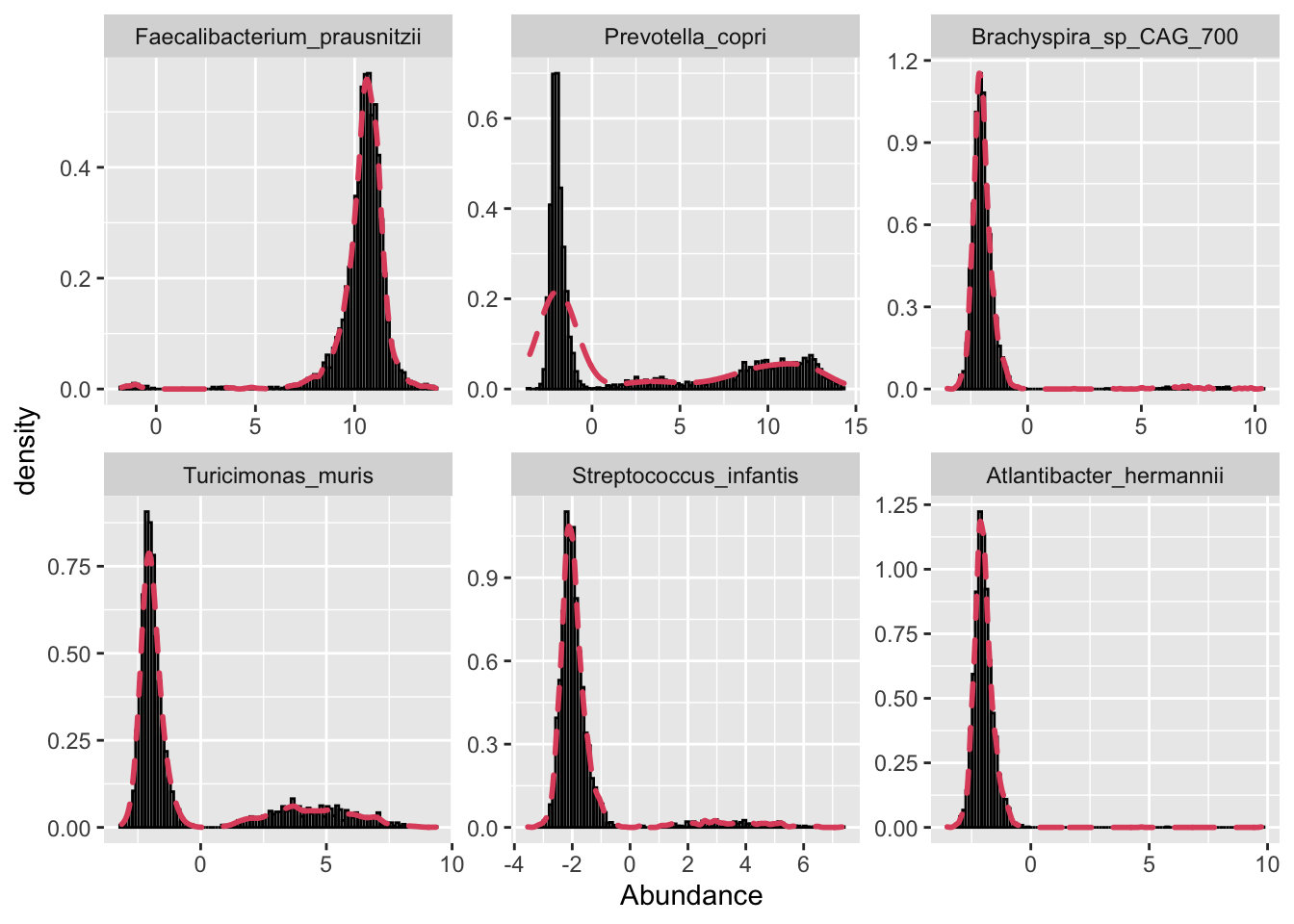
meta_df <- data.frame(sample_data(my_ps)) %>%
  rownames_to_column(var = "seq_id") %>%
  select(seq_id, age, gender, BMI) %>%
  mutate(seq_id = gsub("\\-", ".", seq_id))

otu_tab <- data.frame(otu_table(my_ps)) %>%
  t(.) %>%
  data.frame(.) %>%
  rownames_to_column(var = "seq_id")

mydata <- left_join(meta_df, otu_tab)
rm(meta_df, otu_tab, my_OTUs)


mydata %>%
  mutate(age_bin = cut_number(age, 7),
         bmi_bin = cut_number(BMI, 7)) %>%
  group_by(age_bin, bmi_bin, gender) %>%
  summarise(mean = mean(Prevotella_copri),
            sd = sd(Prevotella_copri)) %>%
  na.omit(.) %>%
  ungroup() %>%
  ggplot(data = ., aes(x = mean, y = sd)) +
    geom_point() +
  labs(x = "\nMean", y = "SD\n") +
  ggtitle("Prevotella_copri")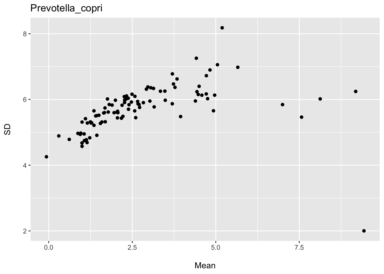
mydata %>%
  mutate(age_bin = cut_number(age, 7),
         bmi_bin = cut_number(BMI, 7)) %>%
  group_by(age_bin, bmi_bin, gender) %>%
  summarise(mean = mean(Streptococcus_infantis),
            sd = sd(Streptococcus_infantis)) %>%
  na.omit(.) %>%
  ungroup() %>%
  ggplot(data = ., aes(x = mean, y = sd)) +
  geom_point() +
  labs(x = "\nMean", y = "SD\n") +
  ggtitle("Streptococcus_infantis")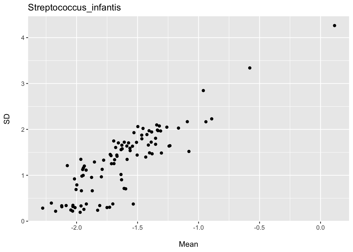
Obtaining population associations
Here I fit the linear model to the six species in the full dataset to obtain values that will serve as the “true” population values of interest.
m1 <- lm(Faecalibacterium_prausnitzii ~ age + gender + BMI, data = mydata)
m2 <- lm(Prevotella_copri ~ age + gender + BMI, data = mydata)
m3 <- lm(Brachyspira_sp_CAG_700 ~ age + gender + BMI, data = mydata)
m4 <- lm(Turicimonas_muris ~ age + gender + BMI, data = mydata)
m5 <- lm(Streptococcus_infantis ~ age + gender + BMI, data = mydata)
m6 <- lm(Atlantibacter_hermannii ~ age + gender + BMI, data = mydata)

a <- tidy(m1)[2:4, 1:2] %>% rename("F.prausnitzii" = "estimate")
b <- tidy(m2)[2:4, 1:2] %>% rename("P.copri" = "estimate")
c <- tidy(m3)[2:4, 1:2] %>% rename("B.sp_CAG_700" = "estimate")
d <- tidy(m4)[2:4, 1:2] %>% rename("T.muris" = "estimate")
e <- tidy(m5)[2:4, 1:2] %>% rename("S.infantis" = "estimate")
f <- tidy(m6)[2:4, 1:2] %>% rename("A.hermannii" = "estimate")

pop_values <- left_join(a, b)
pop_values <- left_join(pop_values, c)
pop_values <- left_join(pop_values, d)
pop_values <- left_join(pop_values, e)
pop_values <- left_join(pop_values, f)

pop_values
## # A tibble: 3 × 7
## term F.prausnitzii P.copri B.sp_CAG_700 T.muris S.infantis A.hermannii
## <chr> <dbl> <dbl> <dbl> <dbl> <dbl> <dbl>
## 1 age -0.00659 -0.0349 -0.00870 -0.0139 -0.00550 -0.00779
## 2 gendermale 0.185 1.29 0.129 -0.183 0.0261 0.0915
## 3 BMI 0.00483 0.0414 -0.00314 -0.00120 0.00702 0.00411rm(a, b, c, d, e, f, m1, m2, m3, m4, m5, m6)Assessing the sample size required for 95% coverage
Now the actual work.
To determine how large a sample would be needed for the CLT to provide reliable results, I draw 1,000 samples of various sizes from n=25 to n=500 for each species and capture the proportion of times the model 95% CI contains the true population value.
These functions are ugly. I know I could have passed the species name and saved some typing, but this was quick and let me get some results up and running.
First, let’s start with the abundant species F.prausnitzii and P.copri. We see these common members of the stool microbiome often.
get_coverage_f <- function(n_samples, age_pop_val, gender_pop_val, bmi_pop_val){
  df <- sample_n(mydata, size = n_samples)
  m <- lm(Faecalibacterium_prausnitzii ~ age + gender + BMI, data = df)
  m_out <- tidy(m, conf.int = TRUE)[2:4, ]

  age_out <- m_out %>%
    filter(term == "age") %>%
    mutate(pop_val = age_pop_val,
           cover = ifelse(between(pop_val, conf.low, conf.high), 1, 0))

  gender_out <- m_out %>%
    filter(term == "gendermale") %>%
    mutate(pop_val = gender_pop_val,
           cover = ifelse(between(pop_val, conf.low, conf.high), 1, 0))

  bmi_out <- m_out %>%
    filter(term == "BMI") %>%
    mutate(pop_val = bmi_pop_val,
           cover = ifelse(between(pop_val, conf.low, conf.high), 1, 0))

  df_out <- bind_rows(age_out, gender_out, bmi_out) %>%
    select(term, cover)

  return(df_out)
}

f_n25 <- replicate(1000, get_coverage_f(n_samples = 25, age_pop_val = -0.00659, gender_pop_val = 0.185, bmi_pop_val = 0.00483), simplify = FALSE) %>%
  bind_rows(., .id = "column_label") %>%
  pivot_wider(names_from = term, values_from = cover) %>%
  mutate(n = 25)

f_n50 <- replicate(1000, get_coverage_f(n_samples = 50, age_pop_val = -0.00659, gender_pop_val = 0.185, bmi_pop_val = 0.00483), simplify = FALSE) %>%
  bind_rows(., .id = "column_label") %>%
  pivot_wider(names_from = term, values_from = cover) %>%
  mutate(n = 50)

f_n100 <- replicate(1000, get_coverage_f(n_samples = 100, age_pop_val = -0.00659, gender_pop_val = 0.185, bmi_pop_val = 0.00483), simplify = FALSE) %>%
  bind_rows(., .id = "column_label") %>%
  pivot_wider(names_from = term, values_from = cover) %>%
  mutate(n = 100)

f_n200 <- replicate(1000, get_coverage_f(n_samples = 200, age_pop_val = -0.00659, gender_pop_val = 0.185, bmi_pop_val = 0.00483), simplify = FALSE) %>%
  bind_rows(., .id = "column_label") %>%
  pivot_wider(names_from = term, values_from = cover) %>%
  mutate(n = 200)

f_n300 <- replicate(1000, get_coverage_f(n_samples = 300, age_pop_val = -0.00659, gender_pop_val = 0.185, bmi_pop_val = 0.00483), simplify = FALSE) %>%
  bind_rows(., .id = "column_label") %>%
  pivot_wider(names_from = term, values_from = cover) %>%
  mutate(n = 300)

f_n400 <- replicate(1000, get_coverage_f(n_samples = 400, age_pop_val = -0.00659, gender_pop_val = 0.185, bmi_pop_val = 0.00483), simplify = FALSE) %>%
  bind_rows(., .id = "column_label") %>%
  pivot_wider(names_from = term, values_from = cover) %>%
  mutate(n = 400)

f_n500 <- replicate(1000, get_coverage_f(n_samples = 500, age_pop_val = -0.00659, gender_pop_val = 0.185, bmi_pop_val = 0.00483), simplify = FALSE) %>%
  bind_rows(., .id = "column_label") %>%
  pivot_wider(names_from = term, values_from = cover) %>%
  mutate(n = 500)

f_df <- bind_rows(f_n25, f_n50, f_n100, f_n200, f_n300, f_n400, f_n500) %>%
  group_by(n) %>%
  summarise(coverage_age = mean(age),
            coverage_gender = mean(gendermale),
            coverage_bmi = mean(BMI))


get_coverage_prev <- function(n_samples, age_pop_val, gender_pop_val, bmi_pop_val){
  df <- sample_n(mydata, size = n_samples)
  m <- lm(Prevotella_copri ~ age + gender + BMI, data = df)
  m_out <- tidy(m, conf.int = TRUE)[2:4, ]

  age_out <- m_out %>%
    filter(term == "age") %>%
    mutate(pop_val = age_pop_val,
           cover = ifelse(between(pop_val, conf.low, conf.high), 1, 0))

  gender_out <- m_out %>%
    filter(term == "gendermale") %>%
    mutate(pop_val = gender_pop_val,
           cover = ifelse(between(pop_val, conf.low, conf.high), 1, 0))

  bmi_out <- m_out %>%
    filter(term == "BMI") %>%
    mutate(pop_val = bmi_pop_val,
           cover = ifelse(between(pop_val, conf.low, conf.high), 1, 0))

  df_out <- bind_rows(age_out, gender_out, bmi_out) %>%
    select(term, cover)

  return(df_out)
}

p_n25 <- replicate(1000, get_coverage_prev(n_samples = 25, age_pop_val = -0.0349, gender_pop_val = 1.29, bmi_pop_val = 0.0414), simplify = FALSE) %>%
  bind_rows(., .id = "column_label") %>%
  pivot_wider(names_from = term, values_from = cover) %>%
  mutate(n = 25)

p_n50 <- replicate(1000, get_coverage_prev(n_samples = 50, age_pop_val = -0.0349, gender_pop_val = 1.29, bmi_pop_val = 0.0414), simplify = FALSE) %>%
  bind_rows(., .id = "column_label") %>%
  pivot_wider(names_from = term, values_from = cover) %>%
  mutate(n = 50)

p_n100 <- replicate(1000, get_coverage_prev(n_samples = 100, age_pop_val = -0.0349, gender_pop_val = 1.29, bmi_pop_val = 0.0414), simplify = FALSE) %>%
  bind_rows(., .id = "column_label") %>%
  pivot_wider(names_from = term, values_from = cover) %>%
  mutate(n = 100)

p_n200 <- replicate(1000, get_coverage_prev(n_samples = 200, age_pop_val = -0.0349, gender_pop_val = 1.29, bmi_pop_val = 0.0414), simplify = FALSE) %>%
  bind_rows(., .id = "column_label") %>%
  pivot_wider(names_from = term, values_from = cover) %>%
  mutate(n = 200)

p_n300 <- replicate(1000, get_coverage_prev(n_samples = 300, age_pop_val = -0.0349, gender_pop_val = 1.29, bmi_pop_val = 0.0414), simplify = FALSE) %>%
  bind_rows(., .id = "column_label") %>%
  pivot_wider(names_from = term, values_from = cover) %>%
  mutate(n = 300)

p_n400 <- replicate(1000, get_coverage_prev(n_samples = 400, age_pop_val = -0.0349, gender_pop_val = 1.29, bmi_pop_val = 0.0414), simplify = FALSE) %>%
  bind_rows(., .id = "column_label") %>%
  pivot_wider(names_from = term, values_from = cover) %>%
  mutate(n = 400)

p_n500 <- replicate(1000, get_coverage_prev(n_samples = 500, age_pop_val = -0.0349, gender_pop_val = 1.29, bmi_pop_val = 0.0414), simplify = FALSE) %>%
  bind_rows(., .id = "column_label") %>%
  pivot_wider(names_from = term, values_from = cover) %>%
  mutate(n = 500)

p_df <- bind_rows(p_n25, p_n50, p_n100, p_n200, p_n300, p_n400, p_n500) %>%
  group_by(n) %>%
  summarise(coverage_age = mean(age),
            coverage_gender = mean(gendermale),
            coverage_bmi = mean(BMI))

f_df
## # A tibble: 7 × 4
## n coverage_age coverage_gender coverage_bmi
## <dbl> <dbl> <dbl> <dbl>
## 1 25 0.932 0.964 0.955
## 2 50 0.91 0.963 0.937
## 3 100 0.894 0.96 0.956
## 4 200 0.884 0.967 0.96
## 5 300 0.905 0.969 0.966
## 6 400 0.91 0.963 0.975
## 7 500 0.924 0.967 0.972p_df## # A tibble: 7 × 4
## n coverage_age coverage_gender coverage_bmi
## <dbl> <dbl> <dbl> <dbl>
## 1 25 0.959 0.928 0.95
## 2 50 0.949 0.942 0.947
## 3 100 0.964 0.948 0.95
## 4 200 0.968 0.958 0.957
## 5 300 0.96 0.956 0.944
## 6 400 0.973 0.956 0.96
## 7 500 0.967 0.968 0.968These results are interesting. For P.copri we look to have pretty good coverage even with rather small sample sizes.
However, for F.prausnitzii we see that for age the coverage is lower and we might expect that our reported alpha levels, even in failry large samples, are overly optimistic (i.e., closer to .1 than .05).
Now lets look at the “middle” abundant species B.sp_CAG_700 and T.muris
get_coverage_b <- function(n_samples, age_pop_val, gender_pop_val, bmi_pop_val){
  df <- sample_n(mydata, size = n_samples)
  m <- lm(Brachyspira_sp_CAG_700 ~ age + gender + BMI, data = df)
  m_out <- tidy(m, conf.int = TRUE)[2:4, ]

  age_out <- m_out %>%
    filter(term == "age") %>%
    mutate(pop_val = age_pop_val,
           cover = ifelse(between(pop_val, conf.low, conf.high), 1, 0))

  gender_out <- m_out %>%
    filter(term == "gendermale") %>%
    mutate(pop_val = gender_pop_val,
           cover = ifelse(between(pop_val, conf.low, conf.high), 1, 0))

  bmi_out <- m_out %>%
    filter(term == "BMI") %>%
    mutate(pop_val = bmi_pop_val,
           cover = ifelse(between(pop_val, conf.low, conf.high), 1, 0))

  df_out <- bind_rows(age_out, gender_out, bmi_out) %>%
    select(term, cover)

  return(df_out)
}

b_n25 <- replicate(1000, get_coverage_b(n_samples = 25, age_pop_val = -0.00870, gender_pop_val = 0.129, bmi_pop_val = -0.00314), simplify = FALSE) %>%
  bind_rows(., .id = "column_label") %>%
  pivot_wider(names_from = term, values_from = cover) %>%
  mutate(n = 25)

b_n50 <- replicate(1000, get_coverage_b(n_samples = 50, age_pop_val = -0.00870, gender_pop_val = 0.129, bmi_pop_val = -0.00314), simplify = FALSE) %>%
  bind_rows(., .id = "column_label") %>%
  pivot_wider(names_from = term, values_from = cover) %>%
  mutate(n = 50)

b_n100 <- replicate(1000, get_coverage_b(n_samples = 100, age_pop_val = -0.00870, gender_pop_val = 0.129, bmi_pop_val = -0.00314), simplify = FALSE) %>%
  bind_rows(., .id = "column_label") %>%
  pivot_wider(names_from = term, values_from = cover) %>%
  mutate(n = 100)

b_n200 <- replicate(1000, get_coverage_b(n_samples = 200, age_pop_val = -0.00870, gender_pop_val = 0.129, bmi_pop_val = -0.00314), simplify = FALSE) %>%
  bind_rows(., .id = "column_label") %>%
  pivot_wider(names_from = term, values_from = cover) %>%
  mutate(n = 200)

b_df <- bind_rows(b_n25, b_n50, b_n100, b_n200) %>%
    group_by(n) %>%
    summarise(coverage_age = mean(age),
              coverage_gender = mean(gendermale),
              coverage_bmi = mean(BMI))


get_coverage_t <- function(n_samples, age_pop_val, gender_pop_val, bmi_pop_val){
  df <- sample_n(mydata, size = n_samples)
  m <- lm(Turicimonas_muris ~ age + gender + BMI, data = df)
  m_out <- tidy(m, conf.int = TRUE)[2:4, ]

  age_out <- m_out %>%
    filter(term == "age") %>%
    mutate(pop_val = age_pop_val,
           cover = ifelse(between(pop_val, conf.low, conf.high), 1, 0))

  gender_out <- m_out %>%
    filter(term == "gendermale") %>%
    mutate(pop_val = gender_pop_val,
           cover = ifelse(between(pop_val, conf.low, conf.high), 1, 0))

  bmi_out <- m_out %>%
    filter(term == "BMI") %>%
    mutate(pop_val = bmi_pop_val,
           cover = ifelse(between(pop_val, conf.low, conf.high), 1, 0))

  df_out <- bind_rows(age_out, gender_out, bmi_out) %>%
    select(term, cover)

  return(df_out)
}

t_n25 <- replicate(1000, get_coverage_t(n_samples = 25, age_pop_val = -0.0139, gender_pop_val = -0.183, bmi_pop_val = -0.00120), simplify = FALSE) %>%
  bind_rows(., .id = "column_label") %>%
  pivot_wider(names_from = term, values_from = cover) %>%
  mutate(n = 25)

t_n50 <- replicate(1000, get_coverage_t(n_samples = 50, age_pop_val = -0.0139, gender_pop_val = -0.183, bmi_pop_val = -0.00120), simplify = FALSE) %>%
  bind_rows(., .id = "column_label") %>%
  pivot_wider(names_from = term, values_from = cover) %>%
  mutate(n = 50)

t_n100 <- replicate(1000, get_coverage_t(n_samples = 100, age_pop_val = -0.0139, gender_pop_val = -0.183, bmi_pop_val = -0.00120), simplify = FALSE) %>%
  bind_rows(., .id = "column_label") %>%
  pivot_wider(names_from = term, values_from = cover) %>%
  mutate(n = 100)

t_n200 <- replicate(1000, get_coverage_t(n_samples = 200, age_pop_val = -0.0139, gender_pop_val = -0.183, bmi_pop_val = -0.00120), simplify = FALSE) %>%
  bind_rows(., .id = "column_label") %>%
  pivot_wider(names_from = term, values_from = cover) %>%
  mutate(n = 200)

t_df <- bind_rows(t_n25, t_n50, t_n100, t_n200) %>%
  group_by(n) %>%
  summarise(coverage_age = mean(age),
            coverage_gender = mean(gendermale),
            coverage_bmi = mean(BMI))


b_df
## # A tibble: 4 × 4
## n coverage_age coverage_gender coverage_bmi
## <dbl> <dbl> <dbl> <dbl>
## 1 25 0.95 0.964 0.932
## 2 50 0.941 0.961 0.945
## 3 100 0.959 0.976 0.951
## 4 200 0.958 0.957 0.97t_df## # A tibble: 4 × 4
## n coverage_age coverage_gender coverage_bmi
## <dbl> <dbl> <dbl> <dbl>
## 1 25 0.936 0.937 0.927
## 2 50 0.927 0.953 0.936
## 3 100 0.947 0.954 0.927
## 4 200 0.939 0.963 0.934Here the results look a bit more similar, and suggest while the coverage is not terrible at smaller sample sizes, we might need a few hundred samples or so to ensure 95%. I only went to n=200 here since in previous runs it looked about sufficient.
Low abundance species S.infantis and A.hermannii
get_coverage_s <- function(n_samples, age_pop_val, gender_pop_val, bmi_pop_val){
  df <- sample_n(mydata, size = n_samples)
  m <- lm(Streptococcus_infantis ~ age + gender + BMI, data = df)
  m_out <- tidy(m, conf.int = TRUE)[2:4, ]

  age_out <- m_out %>%
    filter(term == "age") %>%
    mutate(pop_val = age_pop_val,
           cover = ifelse(between(pop_val, conf.low, conf.high), 1, 0))

  gender_out <- m_out %>%
    filter(term == "gendermale") %>%
    mutate(pop_val = gender_pop_val,
           cover = ifelse(between(pop_val, conf.low, conf.high), 1, 0))

  bmi_out <- m_out %>%
    filter(term == "BMI") %>%
    mutate(pop_val = bmi_pop_val,
           cover = ifelse(between(pop_val, conf.low, conf.high), 1, 0))

  df_out <- bind_rows(age_out, gender_out, bmi_out) %>%
    select(term, cover)

  return(df_out)
}

s_n25 <- replicate(1000, get_coverage_s(n_samples = 25, age_pop_val = -0.00550, gender_pop_val = 0.0261, bmi_pop_val = 0.00702), simplify = FALSE) %>%
  bind_rows(., .id = "column_label") %>%
  pivot_wider(names_from = term, values_from = cover) %>%
  mutate(n = 25)

s_n50 <- replicate(1000, get_coverage_s(n_samples = 50, age_pop_val = -0.00550, gender_pop_val = 0.0261, bmi_pop_val = 0.00702), simplify = FALSE) %>%
  bind_rows(., .id = "column_label") %>%
  pivot_wider(names_from = term, values_from = cover) %>%
  mutate(n = 50)

s_n100 <- replicate(1000, get_coverage_s(n_samples = 100, age_pop_val = -0.00550, gender_pop_val = 0.0261, bmi_pop_val = 0.00702), simplify = FALSE) %>%
  bind_rows(., .id = "column_label") %>%
  pivot_wider(names_from = term, values_from = cover) %>%
  mutate(n = 100)

s_n200 <- replicate(1000, get_coverage_s(n_samples = 200, age_pop_val = -0.00550, gender_pop_val = 0.0261, bmi_pop_val = 0.00702), simplify = FALSE) %>%
  bind_rows(., .id = "column_label") %>%
  pivot_wider(names_from = term, values_from = cover) %>%
  mutate(n = 200)

s_n300 <- replicate(1000, get_coverage_s(n_samples = 300, age_pop_val = -0.00550, gender_pop_val = 0.0261, bmi_pop_val = 0.00702), simplify = FALSE) %>%
  bind_rows(., .id = "column_label") %>%
  pivot_wider(names_from = term, values_from = cover) %>%
  mutate(n = 300)

s_n400 <- replicate(1000, get_coverage_s(n_samples = 400, age_pop_val = -0.00550, gender_pop_val = 0.0261, bmi_pop_val = 0.00702), simplify = FALSE) %>%
  bind_rows(., .id = "column_label") %>%
  pivot_wider(names_from = term, values_from = cover) %>%
  mutate(n = 400)

s_n500 <- replicate(1000, get_coverage_s(n_samples = 500, age_pop_val = -0.00550, gender_pop_val = 0.0261, bmi_pop_val = 0.00702), simplify = FALSE) %>%
  bind_rows(., .id = "column_label") %>%
  pivot_wider(names_from = term, values_from = cover) %>%
  mutate(n = 500)

s_df <- bind_rows(s_n25, s_n50, s_n100, s_n200, s_n300, s_n400, s_n500) %>%
    group_by(n) %>%
    summarise(coverage_age = mean(age),
              coverage_gender = mean(gendermale),
              coverage_bmi = mean(BMI))


get_coverage_a <- function(n_samples, age_pop_val, gender_pop_val, bmi_pop_val){
  df <- sample_n(mydata, size = n_samples)
  m <- lm(Atlantibacter_hermannii ~ age + gender + BMI, data = df)
  m_out <- tidy(m, conf.int = TRUE)[2:4, ]

  age_out <- m_out %>%
    filter(term == "age") %>%
    mutate(pop_val = age_pop_val,
           cover = ifelse(between(pop_val, conf.low, conf.high), 1, 0))

  gender_out <- m_out %>%
    filter(term == "gendermale") %>%
    mutate(pop_val = gender_pop_val,
           cover = ifelse(between(pop_val, conf.low, conf.high), 1, 0))

  bmi_out <- m_out %>%
    filter(term == "BMI") %>%
    mutate(pop_val = bmi_pop_val,
           cover = ifelse(between(pop_val, conf.low, conf.high), 1, 0))

  df_out <- bind_rows(age_out, gender_out, bmi_out) %>%
    select(term, cover)

  return(df_out)
}

a_n25 <- replicate(1000, get_coverage_a(n_samples = 25, age_pop_val = -0.00779, gender_pop_val = 0.0915, bmi_pop_val = 0.00411), simplify = FALSE) %>%
  bind_rows(., .id = "column_label") %>%
  pivot_wider(names_from = term, values_from = cover) %>%
  mutate(n = 25)

a_n50 <- replicate(1000, get_coverage_a(n_samples = 50, age_pop_val = -0.00779, gender_pop_val = 0.0915, bmi_pop_val = 0.00411), simplify = FALSE) %>%
  bind_rows(., .id = "column_label") %>%
  pivot_wider(names_from = term, values_from = cover) %>%
  mutate(n = 50)

a_n100 <- replicate(1000, get_coverage_a(n_samples = 100, age_pop_val = -0.00779, gender_pop_val = 0.0915, bmi_pop_val = 0.00411), simplify = FALSE) %>%
  bind_rows(., .id = "column_label") %>%
  pivot_wider(names_from = term, values_from = cover) %>%
  mutate(n = 100)

a_n200 <- replicate(1000, get_coverage_a(n_samples = 200, age_pop_val = -0.00779, gender_pop_val = 0.0915, bmi_pop_val = 0.00411), simplify = FALSE) %>%
  bind_rows(., .id = "column_label") %>%
  pivot_wider(names_from = term, values_from = cover) %>%
  mutate(n = 200)

a_n300 <- replicate(1000, get_coverage_a(n_samples = 300, age_pop_val = -0.00779, gender_pop_val = 0.0915, bmi_pop_val = 0.00411), simplify = FALSE) %>%
  bind_rows(., .id = "column_label") %>%
  pivot_wider(names_from = term, values_from = cover) %>%
  mutate(n = 300)

a_n400 <- replicate(1000, get_coverage_a(n_samples = 400, age_pop_val = -0.00779, gender_pop_val = 0.0915, bmi_pop_val = 0.00411), simplify = FALSE) %>%
  bind_rows(., .id = "column_label") %>%
  pivot_wider(names_from = term, values_from = cover) %>%
  mutate(n = 400)

a_n500 <- replicate(1000, get_coverage_a(n_samples = 500, age_pop_val = -0.00779, gender_pop_val = 0.0915, bmi_pop_val = 0.00411), simplify = FALSE) %>%
  bind_rows(., .id = "column_label") %>%
  pivot_wider(names_from = term, values_from = cover) %>%
  mutate(n = 500)

a_df <- bind_rows(a_n25, a_n50, a_n100, a_n200, a_n300, a_n400, a_n500) %>%
  group_by(n) %>%
  summarise(coverage_age = mean(age),
            coverage_gender = mean(gendermale),
            coverage_bmi = mean(BMI))

s_df
## # A tibble: 7 × 4
## n coverage_age coverage_gender coverage_bmi
## <dbl> <dbl> <dbl> <dbl>
## 1 25 0.948 0.961 0.927
## 2 50 0.963 0.966 0.95
## 3 100 0.959 0.963 0.947
## 4 200 0.963 0.96 0.955
## 5 300 0.962 0.97 0.951
## 6 400 0.972 0.971 0.95
## 7 500 0.966 0.966 0.955a_df## # A tibble: 7 × 4
## n coverage_age coverage_gender coverage_bmi
## <dbl> <dbl> <dbl> <dbl>
## 1 25 0.936 0.959 0.918
## 2 50 0.949 0.935 0.929
## 3 100 0.956 0.962 0.95
## 4 200 0.961 0.965 0.96
## 5 300 0.95 0.967 0.957
## 6 400 0.955 0.954 0.956
## 7 500 0.978 0.969 0.976Here again it looks like we might not be that far off in smaller samples, but to ensure 95% coverage, we may need a hundred or more samples.
Overall, these results did not look all that bad for most species even at some of the smaller sample sizes considered. Perhaps this is, in part, why the linear model has shown comparability good performance in some benchmarking studies when examined over a large range of simulated species abundances.
However, coverage was less than 95% for some associations suggesting that even at sample sizes of n=500, p-values may be overly optimistic leading to increased type I error rates (failure to control the stated FDR level is well-known issue for differential abundance testing).
Thus at least for me, while I found these results generally encouraging, it seems prudent to suspect the potential for inflated/optimistic test statistics in smaller microbiome studies when interpreting results.
Session Info
sessionInfo()## R version 4.1.1 (2021-08-10)
## Platform: x86_64-apple-darwin17.0 (64-bit)
## Running under: macOS Catalina 10.15.7
##
## Matrix products: default
## BLAS: /Library/Frameworks/R.framework/Versions/4.1/Resources/lib/libRblas.0.dylib
## LAPACK: /Library/Frameworks/R.framework/Versions/4.1/Resources/lib/libRlapack.dylib
##
## locale:
## [1] en_US.UTF-8/en_US.UTF-8/en_US.UTF-8/C/en_US.UTF-8/en_US.UTF-8
##
## attached base packages:
## [1] parallel stats4 stats graphics grDevices utils datasets
## [8] methods base
##
## other attached packages:
## [1] broom_0.7.9 microbiome_1.14.0
## [3] phyloseq_1.36.0 forcats_0.5.1
## [5] stringr_1.4.0 dplyr_1.0.7
## [7] purrr_0.3.4 readr_2.0.2
## [9] tidyr_1.1.4 tibble_3.1.5
## [11] ggplot2_3.3.5 tidyverse_1.3.1
## [13] curatedMetagenomicData_3.0.10 TreeSummarizedExperiment_2.0.3
## [15] Biostrings_2.60.2 XVector_0.32.0
## [17] SingleCellExperiment_1.14.1 SummarizedExperiment_1.22.0
## [19] Biobase_2.52.0 GenomicRanges_1.44.0
## [21] GenomeInfoDb_1.28.4 IRanges_2.26.0
## [23] S4Vectors_0.30.2 BiocGenerics_0.38.0
## [25] MatrixGenerics_1.4.3 matrixStats_0.61.0
##
## loaded via a namespace (and not attached):
## [1] readxl_1.3.1 backports_1.2.1
## [3] AnnotationHub_3.0.2 BiocFileCache_2.0.0
## [5] plyr_1.8.6 igraph_1.2.7
## [7] lazyeval_0.2.2 splines_4.1.1
## [9] BiocParallel_1.26.2 digest_0.6.28
## [11] foreach_1.5.1 htmltools_0.5.2
## [13] fansi_0.5.0 magrittr_2.0.1
## [15] memoise_2.0.0 cluster_2.1.2
## [17] tzdb_0.1.2 modelr_0.1.8
## [19] colorspace_2.0-2 blob_1.2.2
## [21] rvest_1.0.2 rappdirs_0.3.3
## [23] haven_2.4.3 xfun_0.29
## [25] crayon_1.4.1 RCurl_1.98-1.5
## [27] jsonlite_1.7.2 survival_3.2-11
## [29] iterators_1.0.13 ape_5.5
## [31] glue_1.4.2 gtable_0.3.0
## [33] zlibbioc_1.38.0 DelayedArray_0.18.0
## [35] Rhdf5lib_1.14.2 scales_1.1.1
## [37] DBI_1.1.1 Rcpp_1.0.7
## [39] xtable_1.8-4 tidytree_0.3.5
## [41] bit_4.0.4 httr_1.4.2
## [43] ellipsis_0.3.2 farver_2.1.0
## [45] pkgconfig_2.0.3 sass_0.4.0
## [47] dbplyr_2.1.1 utf8_1.2.2
## [49] labeling_0.4.2 tidyselect_1.1.1
## [51] rlang_0.4.12 reshape2_1.4.4
## [53] later_1.3.0 AnnotationDbi_1.54.1
## [55] munsell_0.5.0 BiocVersion_3.13.1
## [57] cellranger_1.1.0 tools_4.1.1
## [59] cachem_1.0.6 cli_3.1.0
## [61] generics_0.1.1 RSQLite_2.2.8
## [63] ExperimentHub_2.0.0 ade4_1.7-18
## [65] evaluate_0.14 biomformat_1.20.0
## [67] fastmap_1.1.0 yaml_2.2.1
## [69] knitr_1.36 bit64_4.0.5
## [71] fs_1.5.0 KEGGREST_1.32.0
## [73] nlme_3.1-152 mime_0.12
## [75] xml2_1.3.2 compiler_4.1.1
## [77] rstudioapi_0.13 filelock_1.0.2
## [79] curl_4.3.2 png_0.1-7
## [81] interactiveDisplayBase_1.30.0 reprex_2.0.1
## [83] treeio_1.16.2 bslib_0.3.1
## [85] stringi_1.7.5 highr_0.9
## [87] blogdown_1.7 lattice_0.20-44
## [89] Matrix_1.3-4 vegan_2.5-7
## [91] permute_0.9-5 multtest_2.48.0
## [93] vctrs_0.3.8 pillar_1.6.4
## [95] lifecycle_1.0.1 rhdf5filters_1.4.0
## [97] BiocManager_1.30.16 jquerylib_0.1.4
## [99] data.table_1.14.2 bitops_1.0-7
## [101] httpuv_1.6.3 R6_2.5.1
## [103] bookdown_0.24 promises_1.2.0.1
## [105] codetools_0.2-18 MASS_7.3-54
## [107] assertthat_0.2.1 rhdf5_2.36.0
## [109] withr_2.4.2 GenomeInfoDbData_1.2.6
## [111] mgcv_1.8-36 hms_1.1.1
## [113] grid_4.1.1 rmarkdown_2.11
## [115] Rtsne_0.15 shiny_1.7.1
## [117] lubridate_1.8.0